16 Models for non-independence – linear mixed models
Probably no chapter in this book is more important for the best-practice analysis of experimental data than this chapter. Why? Because many if not most experimental data violates the assumption of independence and any analysis using standard t-tests and ANOVA will always lead to quantitative error in inference (confidence intervals and p-values) and often lead to qualitative errors in inference (statements about “significance”). Standard analysis of non-independent data can lead to absurdly liberal inference (the p-values are far lower than the data support), but can also lead to moderately conservative inference (the p-values are higher than the data supports). Liberal inference generates false discovery and lures researchers down dead-end research pathways. Conservative inference steers researchers away from true discovery.
Linear Mixed Models are an extension of linear models that appropriately adjust inferential statistics for non-independent data. Paired t-tests and Repeated Measures ANOVA are classical tests that are special cases of linear mixed models. Linear mixed models are more flexible than these classical tests because the models can include added covariates or more complex models generally. And, linear mixed models can be extended to Generalized Linear Mixed Models for counts, binary responses, skewed responses, and ratios.
Before introducing experimental designs that generate non-independent data and the models used to analyze these, let’s explore two ubiquitous examples, one that leads to liberal inference and one that leads to conservative inference.
16.1 Liberal inference from pseudoreplication
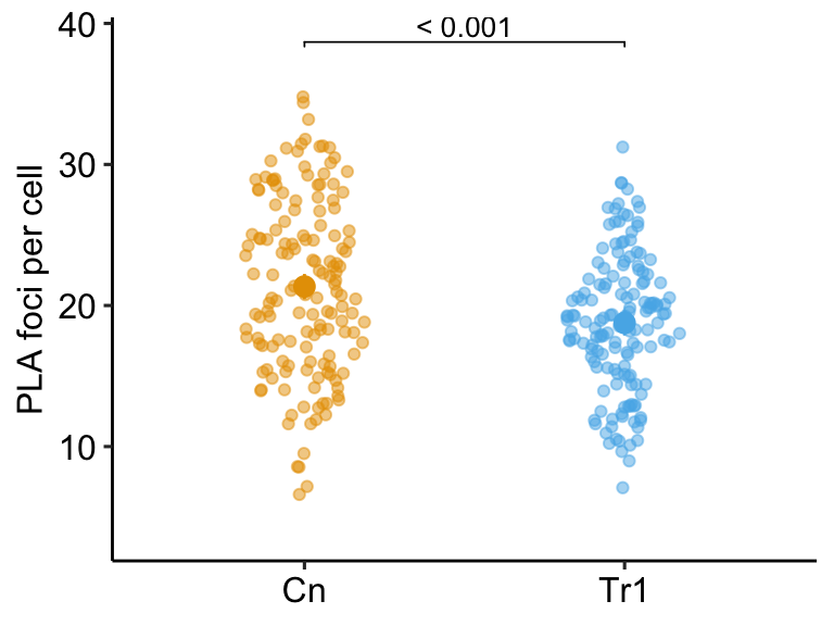
Researchers are interested in regulation and repair of DNA double-stranded breaks and use a proximity ligation assay (PLA) of HeLa cells to investigate the number of damage response events (“foci”) per cell with and without an inhibitor of transcription elongation (DRB). The number of foci in each of fifty cells per treatment is measured. The experiment is replicated three times. The researchers use a t-test to compare the effect of DRB on foci count and naively include all measures in the analysis.
What is naive about the analysis? The fifty measures per cell are technical replicates and the values within a cell are not independent of each other because they share aspects of cell environment not shared by values in other cells. Including technical replicates in an analysis without accounting for this non-independence is a kind of pseudoreplication
To show how this naive analysis results in extremely liberal inference and an increase in false discovery, I simulate this experiment using a case in which there is no effect of DRB treatment, so a low p-value indicates a false-discovery. The simulation is simplified with the two following conditions: 1) the model pretends that count data are normally distributed (this is because we want to focus on pseudoreplication and not a misspecified distribution) and 2) the model pretends that values from each treatment within an experiment are independent (this is because we want to focus on pseudoreplication).
In this naive analysis of the experiment, the researcher finds an effect of treatment with a p-value of 0.000073 and uses this small p-value to justify a decision to move forward with follow-up experiments. But this low p-value is not supported by the data – this discovery is false. This very small p-value is not an example of a “rare event”. In fact, if the researcher repeats the experiment 1000 times, then the median p-value is 0.000195 and 72.3% of the 1000 p-values lead to the same false discovery if 0.05 is used to make the decision to move forward.
While this example is fake, I see this naive analysis a lot: tumor area of multiple tumors per mouse, islet area of multiple islets per mouse, number of vesicles docked to a membrane in multiple cells per mouse, the number of mitochondria in multiple cells per mouse, the number of neurites in multiple neurons in multiple cells per mouse, etc. etc. Indeed, when I’m looking for examples of pseudoreplication to teach, I just look for figures with a bunch of points per treatment – something similar to this plot of the fake data experiment. Regardless, this is a huge source of false discovery that could disappear overnight.

16.2 Conservative inference from failure to identify blocks
Researchers are investigating the regulation of the differentiation of stem blood cells into osteoclasts, which can cause osteoporosis if overactivated. The researchers randomly sample three mice from 6 litters and use a littermate control design: within a litter, one sib is assigned to control (CN), one to glucortacoid (GC) treatment, and one to buthionine sulphoximine (BSO) treatment. The researchers are investigating the mechanism of GC-induced osteoporosis and if the researcher’s model is correct, then BSO should block this mechanism. The response variable is Bone Mineral Density. Following an ANOVA, the researchers report the unadjusted p-value for each pairwise comparison with the expectation that BSO will reverse the effect of GC on Bone Mineral Density.
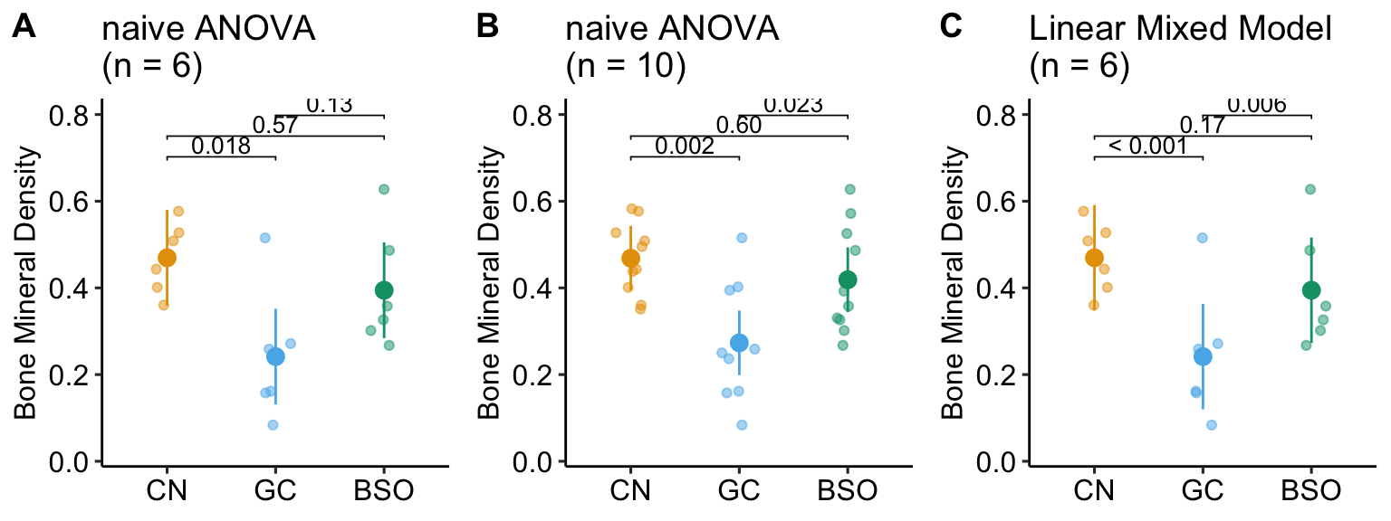
What is naive about the analysis? Any value measured from sibling mice within a litter are not independent of each other because the sibling mice share aspects of genetics and maternal environment not shared by mice in other litters. This shared variance adds correlated noise to data and failure to account for the shared variance will almost always lead to more conservative inference.
In the experiment, the results “looked” like the expected results if the model GC-induced osteoporosis were correct, but the p-value of the focal contrast (BSO - GC) was not < 0.05 (Figure 16.2 A). The researchers expanded the experiment, adding data from four more litters (Figure 16.2 B). Had the researchers analyzed the initial set of data using a statistical model that accounts for the shared variance within a litter (Figure 16.2 C), the researchers would have been satisfied and fewer mice would have been killed, fewer resources used, and more time to pursue continued probing of the mechanism. The statistical model used to take advantage of the littermate control design is a linear-mixed model. An experiment with littermate control is known as a blocked design.
NHST encourages peeking at the data to see if p < 0.05 for a focal contrast, and collecting more data if this isn’t the case. Don’t do this. Peeking makes the p-value non-valid and will increase the false discovery rate. Peeking is a variation of the multiple test problem. In clinical trials there are statistically rigorous methods for peeking, which allows a trial to stop early.
The small p-value in the BSO - GC contrast using a linear mixed model is not an example of a “rare event”. In fact, if the researchers repeated the experiment 1000 times, 89.1% of the BSO - GC p-values using the linear mixed model are less than 0.05 while only 29.9% of the p-values following classical ANOVA are less than 0.05.
While this example is fake, I see this naive analysis a lot – littermate controls is very, very common but other examples are too, including replicated experiments (each experiment is a block). There are certain instances where researchers do recognize non-independence and do use a paired t-test but the vast majority of blocked designs (occurring in almost all experimental biology papers) go unrecognized. This is a huge source of failed discovery that could disappear overnight.
16.3 Introduction to models for non-independent data (linear mixed models)
This chapter is about models for correlated error, including linear models with added random factors, which are known as linear mixed models. In classical hypothesis testing, a paired t-test, repeated measures ANOVA, and mixed-effect ANOVA are equivalent to specific cases of linear mixed models. Linear mixed models are used for analyzing data composed of subsets – or batches – of data that were measured from the “same thing”, such as multiple measures within a mouse, or multiple mice within a litter. Batched data results in correlated error, which violates a key assumption of linear models (and their “which test” equivalents) and muddles statistical inference unless the correlated error is modeled, explicitly or implicitly. In some experimental designs (blocked designs), failure to model the correlated error reduces precision and power, contributing to reduced rates of discovery or confirmation. In other designs (nested designs), failure to model the correlated error results in falsely high precision and low p-values, leading to increased rates of false discovery. The falsely high precision is due to pseudoreplication. I think it’s fair to infer from the experimental biology literature, that experimental biologists don’t recognize the ubiquitousness of batched data and correlated error. This is probably the biggest issue in inference in the field (far more of an issue than say, a t-test on non-normal data).
What do I mean by “batch” and how can correlated error both increase and decrease false discovery? Consider an experiment to measure pancreatic islet area with the experimental factor \(\texttt{treatment}\) with levels “Cn” and “Tr”, where “Cn” is the administration of saline and “Tr” is the administration of a drug believed to disrupt the system. While it may seem like the data from this experiment should be analyzed using a t-test, the best practice statistical model actually depends on the experimental design. Experimental design matters because different designs introduce different patterns of correlated error due to shared genetics and environment. Recall that inference from a linear model (including t-tests and ANOVA) assumes independence (Chapter 8) – that is, each response value has no relationship to any other value, other than that due to treatment. Lack of independence results in patterns of correlation among the residuals, or correlated error.
Something like the first experiment below (Design 1) is the necessary design to use the statistics that have been covered in this book to this point, without extreme violation of the independence assumption. But many (most?) experiments in experimental bench biology do not look like the design in Design 1 below. Instead, many (most?) experiments are variants of Designs 2 and 3, both of which have extreme violations of the independence assumption. Design 2 and its variants result in liberal statistics and increased, false discovery rate but, interestingly, Design 3 and its variants (generally) result in conservative statistics and reduced, true discovery rate.
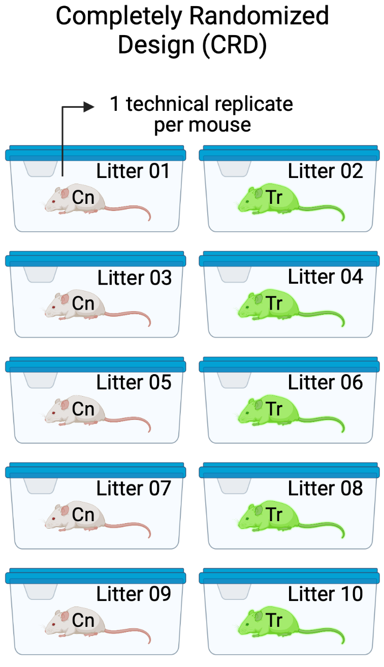
Design 1. The design in Figure 16.3 has a single factor \(\texttt{genotype}\) with two levels (Cn and Tr). Five mice of the same sex, each from a different litter from a unique dam and sire mating, are randomly sampled and assigned to either Cn or Tr. All mice are housed individually (10 cages). The pancreatic tissue from all mice is prepared in a single batch and the area of a single islet is measured from each mouse. The entire experiment is carried out at the same time and each component (tissue preparation, measuring) is carried out by the same person (these could be different people for each component). This is a Completely Randomized Design (CRD). The five replicate mice per treatment are treatment replicates (often called biological replicates in experimental biology). A CRD does not have batched data.
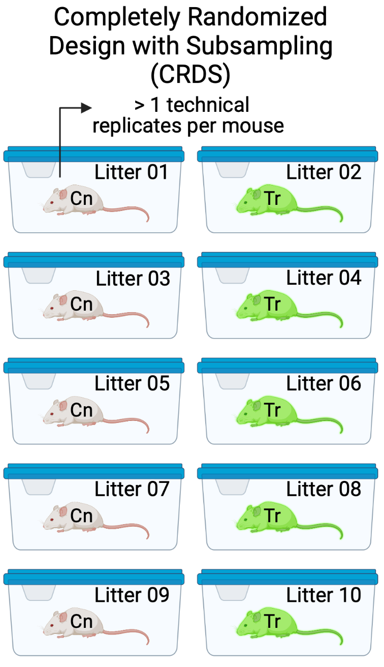
Design 2. The design in Figure 16.4 is exactly like that in Design 1, except that the researchers take ten measures of iselet area per mouse. The ten measures are subsampled replicates. Experimental biologists often call these technical replicates, especially when the multiple measures are taken from the same preparation. Subsampling is a kind of nested design in which one variable is nested within (as opposed to crossed with) another variable. Here, the subsampled variable (subsample_id) is nested within the mouse_id variable. Each mouse is a batch. Each mouse has a unique set of factors that contribute to the error variance of the measures of the response in that mouse. All response measures within a mouse share the component of the error variance unique to that mouse and, as a consequence, the error (residuals) within a mouse are more similar to each other than they are to the residuals between mice
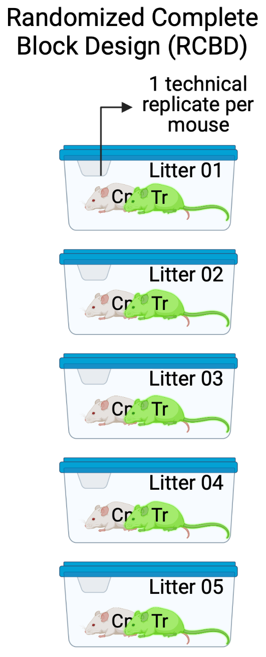
Design 3. In the design in Figure 16.5, two littermates are randomly sampled from five litters, each with a different dam and sire. Within each litter, one mouse is assigned to Cn and a second is assigned to Tr. Each litter is randomly assigned to cage with only a single litter per cage. All other aspects of this design are as in Design 1. This is a Randomized Complete Block Design. The five replicate mice per treatment are the treatment replicates. Each litter/cage combination is a type of batch called a block. A blocked design typically functions to reduce noise in the model fit (this increases power) and to reduce the number of litters and cages needed for an experiment. The two measures of Islet Area within a litter/cage (one per mouse) are not independent of each other. Each cage has two mice from the same litter and these mice share genetic and maternal factors that contribute to mouse anatomy and physiology that are not shared by mice in other litters. Additionally, each cage has a unique set of environmental factors that contribute to the error variance of the measure of the response. Each cage shares a cage-specific history of temperature, humidity, food, light, interactions with animal facilities staff, and behavioral interactions among the mice. All response measures within a litter/cage share the component of the error variance unique to that litter/cage and, as a consequence, the error (residuals) within a litter/cage are more similar to each other than they are to the residuals among litters/cages.
In each of these experiments, there is systematic variation at multiple levels: among treatments due to treatment effects and among batches due to batch effects. Batches come in lots of flavors, including experiment, litter, cage, flask, plate, slide, donor, and individual. The among-treatment differences in means are the fixed effects. The among-batch differences are the random effects. An assumption of modeling random effects is that the batches are a random sample of the batches that could have been sampled. This is often not strictly true as batches are often convenience samples (example: the human donors of the Type 2 diabetes beta cells are those that were in the hospital).
The variation among batches/lack of independence within batches has different consequences on the uncertainty of the estimate of a treatment effect. The batches in Experiment 3 contain both treatments (Cn and Tr). The researcher is interested in the treatment effect but not the variation due to differences among the batches. The batches are nuissance factors that add additional variance to the response, with the consequence that estimates of treatment effects are less precise, unless the variance due to the batches is explicitly modeled. Modeling a batch that contains some or all treatment combinations will increase precision and power.
Batches that contain more than one treatment combination are known as blocks. A block that contains all treatment combinations is a complete block. A block that contains fewer than all combinations is an incomplete block. Including block structure in the design is known as blocking. Blocks are non-experimental factors. Adding a blocking factor to a statistical model is used to increase the precision of an estimated treatment effect. Design 3 is an example of a randomized complete block design.
In Design 2, there are multiple measures per mouse and the design is a Completely Randomized Design with subsampling. The subsampling is not the kind of replication that can be used to infer the among treatment effect because the treatment assignment was not at the level of the subsamples. The treatment replicates are the mice, because it was at this level that treatment assignment was randomized. A statistical analysis of all measures from a subsampled design without modeling the correlated error due to the subsampling is a kind of pseudoreplication. Pseudoreplication results in falsely precise standard errors and false small p-values and, consequently, increased rates of false discovery.
In all of these designs, it is important for the researcher to identify the experimental unit and the measurement unit. The experimental unit is the entity that was randomly assigned the treatment. In all the designs above, the experimental unit is the mouse. In designs 1 and 3, the measurement unit is the mouse. In design 2, the measurement unit is the specific islet that was measured.
In pseudoreplication, the degrees of freedom used to compute the test statistic and the p-value are inflated given the experimental design and research question. An example: A researcher wants to investigate the effect of some protein on mitochondrial biogenesis and designs an experiment with a wildtype (WT) and a conditional knockout (KO) mouse. Mitochondrial counts from twenty cells in one WT mouse and one KO mouse are measured and the researcher uses a t-test to compare counts. The sample size used to compute the standard error in the denominator of the t-value is 20. The t-distribution used to compute the p-value uses 38 df (20 measures times two groups minus two estimated parameters). This is wrong. The df are inflated and the estimate of the standard error of the difference (the denominator of the t-value) is falsely small. The correct sample size for this design is 1 and the correct df is zero. The sample size and df are inflated for this design because the treatment was randomized to mouse and not to cell. Mouse is the experimental unit – the number of experimental units is what gives the degrees of freedom. The df are correct for inference about the two individuals (how compatible are the data and a model of sampling from the same individual?), but not for inference about the effect of genotype. We cannot infer anything about genotype with a sample size of 1, even with 20 measures per mouse, because any effect of treatment is completely confounded with other differences between the two mice.
16.4 Experimental designs in experimental bench biology
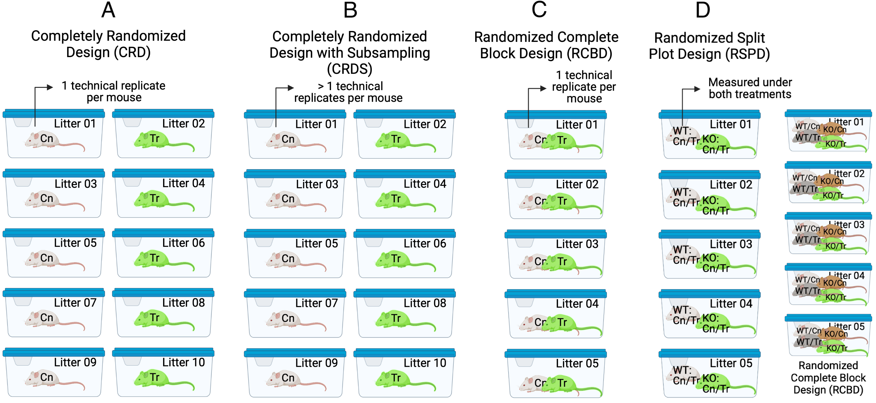
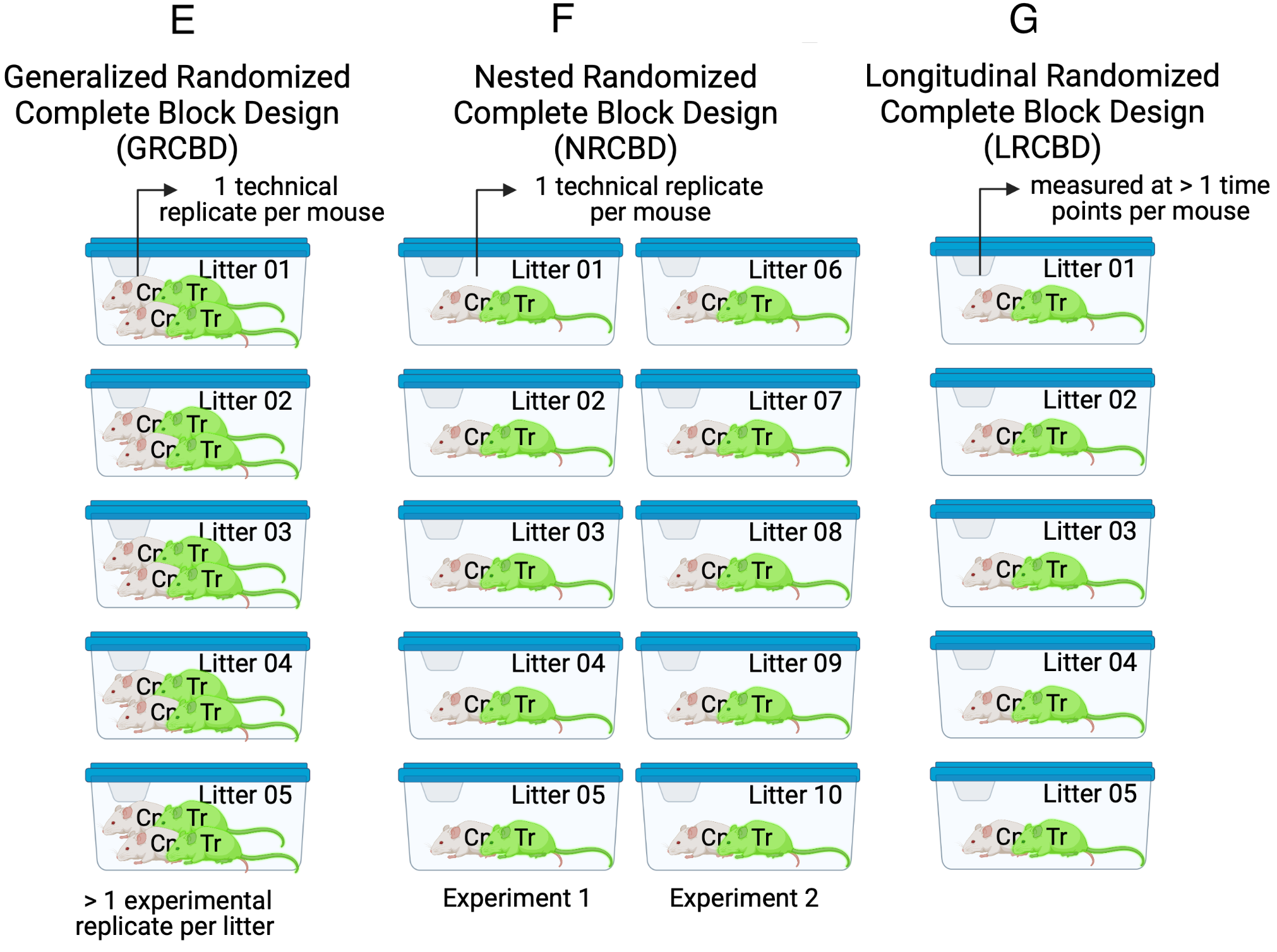
Given the basic principles above, let’s consider the kinds of experimental designs seen in experimental bench biology (Figure 16.6). For each of the experimental designs, I give examples with a certain number of treatments (t), blocks (b), treatment replications (r), and subsampled replications (s).
Notation for models
i = 1..t (treatments)
j = 1..b (blocks)
k = 1..r (treatment replications within a block or within a CRD with no block structure)
m = 1..s (subsamples or technical replicates)
16.4.1 Completely Randomized Design (CRD)
The Completely Randomized Design experiment in Figure 16.6 A has a single factor, \(\texttt{treatment}\) with two levels (“Cn” and “Tr”). Five mice are randomly assigned to each treatment level. Each mouse is bred from a different litter and housed in a separate cage. The researchers measure a single value of the response variable from each mouse. The five replicate mice per treatment are the treatment (biological) replicates. The design is completely randomized because there is no subgrouping due to batches. What kinds of subgrouping does this design avoid?
By using a single mouse per litter, there are no litter batches and subsets of mice don’t share litter effects – common litter responses to the Cn or Tr treatments. Each litter has a unique set of factors that contribute to the error variance of the measure of the response. Siblings from the same dam and sire share more genetic variation than non-siblings and this shared genetic variation contributes to phenotypes (including the response to treatment) that are more likely to be similar to each other than to non-siblings. Siblings from the same litter share the same history of maternal factors (maternal effects, including epigenetic effects) specific to the pregnancy and even the history of events leading up to the pregnancy. This shared non-genetic and epigenetic variation contributes to phenotypes (including the response to treatment) that are more likely to be similar to each other than to non-siblings. All response measures within a litter share the genetic, maternal environmental, and epigenetic components of the error variance unique to that litter and, as a consequence, the error (residuals) within a litter are more similar to each other than they are to the residuals between litters.
By housing each mouse in it’s own cage, there is no cage batch and subsets of mice don’t share cage effects – common cage responses to the Cn or Tr treatments. As stated earlier, each cage has a unique set of factors that contribute to the error variance of the measure of the response. Each cage shares a cage-specific history of temperature, humidity, food, light, interactions with animal facilities staff and behavioral interactions among the mice. All response measures within a cage share the component of the error variance unique to that cage and, as a consequence, the error (residuals) within a cage are more similar to each other than they are to the residuals between cages.
Examples:
- Ten mice from separate litters are sampled. Five mice are randomly assigned to control. Five mice are randomly assigned to treatment. A single measure per mouse is taken. Mouse is the experimental unit. \(t=2\), \(b=0\), \(r=5\), and \(s=1\).
- Ten cell cultures are created. Five cultures are randomly assigned to control and five to treatment. A single measure per culture is taken. Culture is the experimental unit. \(t=2\), \(b=0\), \(r=5\), and \(s=1\).
While most data from experiments in bench biology are analyzed as if the experimental design is a CRD, a good question is, what fraction of these actually are CRD? We know that many (most?) mouse experiments will have batched measures and correlated responses because most experiments are conducted with multiple mice per litter and/or cage (or equivalents in other model systems). Many cell culture data come from multiple replicates of the whole experiment – the experiment functions as a block. And time series experiments include multiple measures on the same experimental unit over time. Except for time series experiments, researchers in experimental bench biology are using almost exclusively statistical tests that assume independence of errors (the tests appropriate for CRDs). How this mismatch between experimental design and statistical practice affects the rate of false and true discovery in cell and molecular biology is a known unknown.
16.4.2 Completely Randomized Design with Subsampling (CRDS) or “Nested Design”
The Completely Randomized Design with Subsampling experiment in Figure 16.6 B is exactly like the CRD except that the researchers measure multiple values of the response variable from each mouse under the same condition (that is, not different in treatment or time). The multiple measures are subsampled (technical) replicates.
- Do not confuse subsampled replicates with measures of the response under different conditions in the same mouse, for example a measure from one brain slice under the control treatment and a measure from a second brain slice under the drug treatment. This example is a kind of Randomized Complete Block Design, which is outlined next and the core design in this chapter.
- Do not confuse subsampled replicates with a measures of the response at different times in the same mouse, for example, the plasma glucose levels at baseline and at five post-baseline time points. This example is a kind of longitudinal design, which is outlined below and more thoroughly in the chapter Linear models for longitudinal experiments.
- Do not confuse subsampled replicates with measures of different response variables from the same mouse, for example measures of the weights of five different skeletal muscles. This example is a kind of multiple response which is addressed xxx.
The technical replicates are a kind of pseudoreplication. The general linear model y ~ treatment fit to these data, including t-tests and traditional ANOVA, will have falsely high precision and falsely low p-values.
Examples:
- Ten mice from separate litters are sampled. Five mice are randomly assigned to control. Five mice are randomly assigned to treatment. Multiple measures per mouse are taken. Example: five measures of Islet Area are measured in each pancreas. Mouse is the experimental unit. Each of the measures is a technical replicate because the treatment is not randomly assigned to each islet but to the whole mouse. \(t=2\), \(b=0\), \(r=5\), and \(s=5\).
- Ten cell cultures are created. Five cultures are randomly assigned to control and five to treatment. Multiple measures per culture are taken. Example: Mitochondrial counts are measured from five cells in each culture. Culture is the experimental unit. Each of the counts is a technical replicate because the treatment is not randomly assigned to each cell but to the whole culture. \(t=2\), \(b=0\), \(r=5\), and \(s=5\).
Notes:
- Subsampling can occur at multiple levels. Example: Ten mice from separate litters are sampled. Five mice are randomly assigned to control. Five mice are randomly assigned to treatment. Five neurons in a slice of brain tissue are identified in each mouse. From each neuron, the length of five dendrite spines are measured. The five measures of spine length are “nested within” neuron and the five neurons are “nested within” mouse. Nested subsampling can quickly lead to massive pseudoreplication and false discovery.
16.4.3 Randomized Complete Block Design (RCBD)
The Randomized Complete Block Design experiment in Figure 16.6 C is similar to the CRD except that all treatment combinations (two here) are randomly assigned to sibling mice within a litter. Here, two mice from each litter are randomly selected and one is randomly assigned to “Cn” and the other to “Tr”. Each litter is randomly assigned to a unique cage. The researchers measure a single value of the response variable from each mouse. The five replicate mice per treatment are the treatment replicates. The litters (or cage) are the blocks. In this design, litter and cage effects are confounded but this has no consequence on the statistical model and inference unless the researchers want to explicitly estimate these effects separately. Compared to the CRD, this design requires fewer resources (five litters instead of ten, five cages instead of ten). Compared to the general linear model fit to data from the CRD (y ~ treatment), including t-tests and traditional ANOVA, the linear mixed model fit to the RCBD has increased precision and power. While many researchers seem to be designing experiments similar to this (“littermate controls”), most are failing to fit a statistical model that accounts for the batching and taking advantage of the increased precision and power.
Examples:
- Ten mice are sampled. In each mouse, one forelimb is assigned to control and the other forelimb is assigned to treatment. Only a single measure on each side is taken. Limb is the experimental unit. Mouse is a block. \(t=2\), \(b=10\), \(r=1\), and \(s=1\).
- Ten litters are sampled. In each litter, one sib is assigned to control and the other sib is assigned to treatment. Only a single measure on each sib is taken. Mouse is the experimental unit. Litter is a block. \(t=2\), \(b=10\), \(r=1\), and \(s=1\).
- Two mice, each from a separate litter are sampled. One is randomly assigned to control and the other to treatment. Only a single measure of the response variable is taken per mouse. The experiment is replicated five times (five different days, each with a newly made set of reagents and machine calibrations). Mouse is the experimental unit. Experiment is a block. \(t=2\), \(b=5\), \(r=1\), and \(s=1\).
16.4.4 Randomized Split Plot Design (RSPD)
The Randomized Split Plot Design experiment in Figure 16.6 D is similar to the RCBD except that there is now a second experimental factor that is crossed with the first experimental factor. An individual mouse acts as single experimental unit for one factor (here, \(\texttt{genotype}\) with levels “WT” and “KO”) but acts as a block for the second experimental factor (here, \(\texttt{treatment}\) with levels “Cn” and “Tr”). The first factor (\(\texttt{genotype}\)) is the main plot – the levels of the factor are randomly assigned to the main plots. The second factor (\(\texttt{treatment}\)) is the subplot – the levels of this factor are randomly assigned to the subplots. \(\texttt{Litter}\) is a replicated block. Also in Figure 16.6 D, a 2 x 2 RCBD with the same two experimental factors is shown for comparison. In the 2 x 2 RCBD, four mice per block (litter) are each randomly assigned one of the 2 x 2 combinations of \(\texttt{genotype}\) and \(\texttt{treatment}\)).
16.4.5 Generalized Randomized Complete Block Design (GRCBD)
The Generalized Randomized Complete Block Design experiment in Figure 16.6 E is similar to the RCBD except that two treatment replicates per block (litter/cage) are assigned.
Important and somewhat not intuitive Because the treatment replicates within a litter share common error variance, these do not act like independent replicates. One consequence of this is, the sample size (\(n\)) is five and not ten (\(litters \times treatment replicates\)). The general linear model y ~ treatment fit to these data, including t-tests and traditional ANOVA, will generally have falsely high precision and falsely low p-values.
16.4.6 Nested Randomized Complete Block Design (NRCBD)
The Nested Randomized Complete Block Design experiment in Figure 16.6 F is similar to the RCBD except that there are now replicated experiments. This is a nested block design with litter (a block) nested within experiment (a block).
16.4.7 Longitudinal Randomized Complete Block Design (LRCBD)
The Longitudinal Randomized Complete Block Design experiment in Figure 16.6 G is similar to the RCBD except that there are multiple measures of the response variable taken, each taken at a different time point, including baseline (time zero).
16.4.8 Variations due to multiple measures of the response variable
Similar to the CRDS above, the other basic designs can include subsampling, resulting in, for example, RCBDS or RSPDS. If there is subsampling within subsampled units, then we can designated these with “SS”, for example RCBDSS.
Similar to the LRCBD above, the other basic designs can include longitudinal sampling, resulting in, for example, LCRD or LRSPD.
16.5 Building the linear (mixed) model for clustered data
Notation
- i = 1..t (treatments)
- j = 1..b (blocks)
- k = 1..r (experimental replications within a block)
- m = 1..s (subsamples or technical replicates)
\[y_i = \beta_0 + \beta_i treatment_i + (\gamma_j block_j) + (\gamma_{ij} block_j treatment_i) + \varepsilon\]
16.6 Statistical models for experimental designs
16.6.1 Models for Completely Randomized Designs (CRD)
lm.crd <- lm(y ~ treatment,
             data = figx)
16.6.2 Models for batched data (CRDS, RCBD, RSPD, GRCBD, NRCBD)
16.6.2.1 Linear models
16.6.2.1.1 fixed effect model
lm.fe <- lm(y ~ treatment + block,
             data = figx)
16.6.2.1.2 linear model of batch means (aggregated linear model)
figx_means <- figx[, .(y = mean(y)),
               by = .(treatment, batch)]
lm.agg <- lm(y ~ treatment,
             data = figx_means)
16.6.2.2 linear mixed models (“random effects” models)
16.6.2.2.1 Random intercept model
lmm.ri <- lmer(y ~ treatment + (1 | block),
              data = figx)
16.6.2.2.2 random interaction intercept model
lmm.rii <-  lmer(y ~ treatment + (1 | block) + (1 | block:treatment),
               data = figx)
16.6.2.2.3 random interaction model with subsampling
lmm.riis <-  lmer(y ~ treatment + (1 | block) + (1 | block:treatment) +
                (1 | block:treatment:replicate),
               data = figx)
16.6.2.2.4 random interaction model for two factor designs
lmm.rii2 <-  lmer(y ~ factor1 * factor2 + (1 | block) + (1 | block:factor1) +
                (1 | block:factor2),
               data = figx)
16.6.2.2.5 random intercept and slope model
lmm.ris <-  lmer(y ~ treatment + (treatment | block),
data = figx)16.6.2.2.7 Split plot model
# factor1 is the main plot
# factor2 is the subplot
# main_plot_id is the replicate ID of the main plot
lmm.sp1 <-  lmer(y ~ factor1 * factor2 + (1 | main_plot_id),
               data = figx)
16.6.2.2.8 Replicated split plot model
# factor1 is the main plot
# factor2 is the subplot
# main_plot_id is the replicate ID of the main plot
lmm.sp2 <-  lmer(y ~ factor1 * factor2 + (1 | main_plot_id) + (1 | main_plot_id:factor1),
               data = figx)

lmm.sp2 <-  lmer(y ~ factor1 * factor2 + main_plot_id + (1 | main_plot_id:factor1),
               data = figx)
# the two versions are numerically equivalent
16.6.2.3 ANOVA models
16.6.2.3.1 Nested ANOVA
# nest_id is the batch containing the subsampled replicates
naov <- aov_4(y ~ treatment + (1 | nest_id),
              fun_aggregate = mean,
              data = figx)
16.6.2.3.2 Univariate repeated measures ANOVA
rmaov.uni <- aov_4(y ~ treatment + (treatment | block),
           include_aov = TRUE,
             data = figx)
# requires the argument model = "univariate" in the emmeans function
16.6.2.3.3 Univariate repeated measures ANOVA for two factor designs
# the factor treatment contains all combinations of factor 1 and factor 2
rmaov.uni1x <- aov_4(y ~ treatment + (treatment | block),
           include_aov = TRUE,
             data = figx)
# requires the argument model = "univariate" in the emmeans function
rmaov.uni2x <- aov_4(y ~ factor1 * factor2 + (factor1 * factor2 | block),
include_aov = TRUE,
data = figx)
# requires the argument model = "univariate" in the emmeans function16.6.2.3.4 Multivariate repeated measures ANOVA
rmaov.mul <- aov_4(y ~ treatment + (treatment | block),
             data = figx)
16.6.2.3.5 Repeated measures ANOVA for Split Plot
# factor1 is the main plot
# factor2 is the subplot
# main_plot_id is the replicate ID of the main plot

rmaov.sp <- aov_4(y ~ factor1 * factor2 + (factor1 | main_plot_id),
             data = figx)
16.6.2.3.6 Pairwise paired, t-tests
ppttm <- pptt(y ~ treatment + (1 | block),
             data = figx)
16.7 Which model and why?
16.7.1 CRD
- lm.crd
16.7.2 CRDS
- lmm.ri – random intercept model
- lm.agg – linear model of batch means
- naov – nested ANOVA
Notes
- These are numerically equivalent if the design is balanced
16.7.3 RCBD
16.7.3.1 Statistical models for single factor RCBD
- lm.fe – fixed effect model
- lmm.ri – random intercept model
- lmm.ce – lmm for correlated error
- rmaov.mul – multivariate RM-ANOVA
- rmaov.uni1 – univariate RM-ANOVA
- pptt – pairwise, paired t-test
(Cannot use lmm.ris or lmm.rii because there is no replication of each block:treatment combination.)
Equivalent models if the design is balanced
- If the number of treatments = 2, all six methods are numerically equivalent. A paired t-test is a special case of a linear mixed model.
- If the number of treatments > 2, then
- lmm.ri, lm.fe, and rmaov.uni are equivalent
- lmm.ce, rmaov.mul, ppttm result in the same estimates and SE. The emmeans::contrast() default df of lmm.ce are higher than the rmaov.mul/ppttm df, so the CIs and p-values of lmm.ce are less conservative.
If the design is not balanced (at least one block:treatment combination is missing)
- If a treatment within a block is missing, the whole block is deleted in the rmoav models. This reduces power (the loss of power depends partly on the number of missing values).
- If a treatment within a block is missing, the block is deleted only in the comparisons including the missing treatment in the pairwise, paired t-tests. This makes ppttm more powerful than rmaov.mul
- No blocks are deleted in linear mixed models.
Some general notes
- the lmm models are very flexible – covariates can be added or these can be used as generalized lmms for non-normal distributions.
- the lmm models sometimes fail to converge, especially with small samples (small number of blocks) or if the among-block component or block:treatment components of variance are small.
16.7.3.2 Additional models for two factor RCBD
- lmm.rii2 – random interaction intercept model with each factor:block intercept
- rmaov.uni2 – two-factor univariate RM-ANOVA
Equivalent models if the design is balanced
- lm.fe, lmm.ri, and rmaov.uni1 are equivalent
- lmm.rii2 and rmaov.uni2 are equivalent
- rmaov.mul and ppttm are equivalent
- lmm.ce is equivalent to rmaov.mul/ppttm, depending on how one models the df
16.7.3.3 Which model and why
- For single factor RCBD with only two treatment levels, all models are the same if the design is balanced so it doesn’t matter. If the design is unbalanced, lmm.ri will have more power because no block:treatment combinations are excluded.
- For single factor RCBD with more than two treatment levels, lmm.ce/rmaov.mul/ppttm control type I error well
- For two factor RCBD…
16.7.4 RSPD
- lmm.sp1 - random intercept model for CRD split plot designs
- lmm.sp2 - random interaction intercept model of RCBD split plot designs
- rmaov.sp - repeated measures ANOVA for a split plot design
16.7.5 RCBDS
- lmm.ris – random intercept and slopes model
- lmm.rii – random interaction intercept model
- lmm.ri – random intercept model on batch means
- lmm.ce – lmm for correlated error on batch means
- rmaov.mul – multivariate RM-ANOVA
- rmaov.uni – univariate RM-ANOVA
- pptt – pairwise, paired t-test
Notes
- lmm.ris is the “maximal model” – it fits the most parameters and has the fewest assumptions. lmm.ri on the full data is the minimal model. I’m not recommending this at all as this is pseudoreplication and will result in very anti-conservative inference. lmm.rii is less conservative than lmm.ris (and makes more assumptions).
- lmm.ri and lmm.ce here are the models for RCBD designs but using the aggregated data - that is the subsampled replicates within a batch (block:treatment combination) are averaged.
- If design is balanced
- lmm.ris and rmaov.mul result in same estimates, SE, CIs, and p-values
- lmm.rii, lmm.ri, and rmaov.uni result in same estimates, SE, CIs, and p-values
- lmm.ce has same estimates and SE as lmm.ris/rmaov.mul but more df so less conservative
- If a treatment within a block is missing, the whole block is deleted in the RM-ANOVA models. This reduces power
- the lmm models are very flexible – covariates can be added or these can be used as generalized lmms for non-normal distributions.
- the lmm models, and especially lmm.ce and lmm.ris, sometimes (often?) fail to converge, especially with small samples (small number of blocks) or if within block correlation is small
- lmm.ri, lmm.rii, and rmaov.uni will be less conservative (more power but at higher type I error/false positive rate)
Best practices
- If balanced and no covariates then use lmm.ris/lmm.ce/rmaov.mul if discovery is expensive (want to avoid false positives) or lmm.rii/rmaov.uni/lmm.ri if discovery is cheap (can afford false positives). lmm.ce is less conservative than lmm.ris/rmaov.mul. Use lmm.ris if interested in the variance at different levels and/or covariance structure.
- If unbalanced, or if there are covariates, then start with lmm.ris or lmm.ce. Use lmeControl if lmm.ce fails. If these fail, go to 1.
16.7.6 GRCBD
- lmm.ris – random intercept and slopes model
- lmm.rii – random interaction intercept model
- lmm.ri – random intercept model on block:treatment means
- lmm.ce – lmm for correlated error on block:treatment means
- rmaov.mul – multivariate RM-ANOVA
- rmaov.uni – univariate RM-ANOVA
- lm.fe – fixed effect model on all data
- pptt – pairwise, paired t-test on block:treatment means
16.7.7 GRCBDS
- lmm.ris – random intercept and slopes model
- lmm.rii – random interaction intercept model
- lmm.ri – random intercept model on block:treatment means
- lmm.ce – lmm for correlated error on block:treatment means
- rmaov.mul – multivariate RM-ANOVA
- rmaov.uni – univariate RM-ANOVA
- lm.fe – fixed effect model on all block:treatment:rep means
- pptt – pairwise, paired t-test on block:treatment:rep means
16.8 Example 1: CRD with subsampling (classical equivalent: Nested ANOVA)
Source article: A new mouse model of Charcot-Marie-Tooth 2J neuropathy replicates human axonopathy and suggest alteration in axo-glia communication
Published methods: Nested ANOVA
Fig: 5b
Design: 3 x 1 CRDS
| genotype | mouse | N |
|---|---|---|
| WT | WT 1 | 90 |
| WT | WT 2 | 58 |
| WT | WT 3 | 60 |
| WT | WT 4 | 92 |
| TM/+ | TM/+ 1 | 76 |
| TM/+ | TM/+ 2 | 52 |
| TM/+ | TM/+ 3 | 66 |
| TM/TM | TM/TM 1 | 78 |
| TM/TM | TM/TM 2 | 74 |
| TM/TM | TM/TM 3 | 70 |
| TM/TM | TM/TM 4 | 48 |
| TM/TM | TM/TM 5 | 54 |
16.8.1 Model fit and inference
16.8.1.1 Model fit
fig5b_lmm <- lmer(caspr_length ~ genotype + (1 | mouse), data = fig5b)Notes
- This model is called a “random intercept” model. The factor \(\texttt{mouse}\) is a random factor and is added to the model as a random intercept. Random factors are added inside parentheses. A random intercept is specified with a 1 in front of the bar.
16.8.1.2 Inference
fig5b_lmm_emm <- emmeans(fig5b_lmm, specs = "genotype")
fig5b_lmm_pairs <- contrast(fig5b_lmm_emm, method = "revpairwise", adjust = "tukey") |>
  summary(infer = TRUE)
fig5b_lmm_pairs |>
  kable(digits = c(1,2,2,1,2,2,1,4)) |>
kable_styling()| contrast | estimate | SE | df | lower.CL | upper.CL | t.ratio | p.value |
|---|---|---|---|---|---|---|---|
| (TM/+) - WT | 0.48 | 0.16 | 8.9 | 0.03 | 0.93 | 3.0 | 0.0387 |
| (TM/TM) - WT | 0.49 | 0.14 | 8.8 | 0.09 | 0.88 | 3.4 | 0.0192 |
| (TM/TM) - (TM/+) | 0.01 | 0.16 | 9.2 | -0.43 | 0.44 | 0.0 | 0.9990 |
Notes
- I would not adjust the p-values (see Chapter 12) but I have adjusted using Tukey HSD to compare to researcher’s results in next section
16.8.1.3 Plot the model
set.seed(1)
ggptm(fig5b_lmm, fig5b_lmm_emm, fig5b_lmm_pairs,
      show_nest_data = TRUE,
      nest_id = "mouse",
      hide_pairs = 3,
      y_label = "Caspr Length (µm)",
      palette = pal_okabe_ito_blue)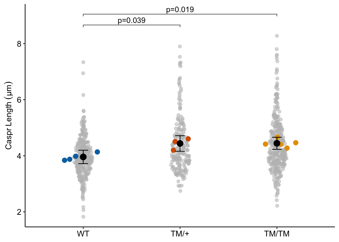
16.8.2 What the researchers did: Classical nested ANOVA
fig5b_aov <- aov_4(caspr_length ~ genotype + (1 | mouse),
                   fun_aggregate = mean,
                   data = fig5b)
fig5b_aov_emm <- emmeans(fig5b_aov, specs = "genotype")
fig5b_aov_pairs <- contrast(fig5b_aov_emm, method = "revpairwise", adjust = "tukey") |>
  summary(infer = TRUE) |>
  data.table()
fig5b_aov_pairs |>
  kable(digits = c(1,2,2,1,2,2,1,4)) |>
kable_styling()| contrast | estimate | SE | df | lower.CL | upper.CL | t.ratio | p.value |
|---|---|---|---|---|---|---|---|
| (TM/+) - WT | 0.49 | 0.17 | 9 | 0.02 | 0.95 | 2.9 | 0.0401 |
| (TM/TM) - WT | 0.49 | 0.15 | 9 | 0.08 | 0.90 | 3.4 | 0.0204 |
| (TM/TM) - (TM/+) | 0.00 | 0.16 | 9 | -0.44 | 0.45 | 0.0 | 0.9996 |
Notes
- If the design is balanced (all units have the same sample size), classical nested ANOVA and the linear mixed model with a random intercept are equivalent.
- In general, ANOVA doesn’t handle lack of balance well (different sample sizes per unit). If there were the same number of measures per mouse, The t and p values of this nested anova would be the same as these values fit by the linear mixed model. As is, the t value is slightly smaller and the p-value is slightly larger in the nested ANOVA.
16.8.3 What if the researchers had ignored the non-independence?
fig5b_lm <- lm(caspr_length ~ genotype, data = fig5b)
fig5b_lm_emm <- emmeans(fig5b_lm, specs = "genotype")
fig5b_lm_pairs <- contrast(fig5b_lm_emm, method = "revpairwise", adjust = "tukey") |>
  summary(infer = TRUE) |>
  data.table()
fig5b_lm_pairs[, p.value := format(p.value, digits = 3)]
fig5b_lm_pairs |>
  kable(digits = c(1,2,2,1,2,2,1,2)) |>
kable_styling()| contrast | estimate | SE | df | lower.CL | upper.CL | t.ratio | p.value |
|---|---|---|---|---|---|---|---|
| (TM/+) - WT | 0.46 | 0.08 | 815 | 0.27 | 0.66 | 5.6 | 7.29e-08 |
| (TM/TM) - WT | 0.48 | 0.07 | 815 | 0.31 | 0.65 | 6.7 | 1.15e-10 |
| (TM/TM) - (TM/+) | 0.02 | 0.08 | 815 | -0.17 | 0.21 | 0.2 | 9.79e-01 |
Notes
- The p-values are extremely small because the model “thinks” the data are independent. This is an example of pseudoreplication – using technical replicates as treatment replicates.
16.8.4 A deeper dive into the random intercepts
Remember, intercepts are means. A random intercept model computes a mean for each level of the random factor, so here, the model is computing a mean for each mouse. The mouse means are not the mean you would compute using a calculator. Instead the modeled mean of each mouse within a treatment is a little closer to the treatment mean than the sample mean of each mouse. That is, the deviation between the mouse mean and the treatment mean are “shrunk toward zero”.
It is easy to show these shrunken estimates of the cluster means. Here are the modeled means of each WT mouse, and the deviation from the modeled treatment mean.
lmm_means_table <- data.table(
  mouse = unique(fig5b[genotype == "WT", mouse]),
  intercept = coef(fig5b_lmm)$mouse[1:4, "(Intercept)"])
lmm_means_table[, deviation := intercept - coef(summary(fig5b_lmm))[1, "Estimate"]]
lmm_means_table
mouse intercept deviation
<fctr> <num> <num>
1: WT 1 3.872542 -0.08586488
2: WT 2 4.137722 0.17931496
3: WT 3 3.839612 -0.11879463
4: WT 4 3.983751 0.02534454Here are the sample means of each WT mouse and the deviation from the treatment mean
sample_means_table <- fig5b[genotype == "WT", .(mean = (mean(caspr_length))), by = .(mouse)]
sample_means_table[, deviation := mean - mean(mean)]
sample_means_table
mouse mean deviation
<fctr> <num> <num>
1: WT 1 3.850525 -0.11038077
2: WT 2 4.209068 0.24816221
3: WT 3 3.793921 -0.16698438
4: WT 4 3.990108 0.0292029316.9 Example 2: RCBD with 2 groups (classical equivalent: paired t-test)
Source Figure: Fig 2C upper left (NR4A1 using CAR)
Response variable: NR4A expression measured as MFI (mean flourescence intensity)
Treatment: CAR PD-1hi TIM3hi TILs, CAR PD-1hi TIM3lo TILs (so differ in density of TIM3 receptors)
Experimental Design: Randomized Complete Block Design (RCBD). Three preparations (experiments). Experiment is the block.
Background: CAR-T are T cells expressing chimeric antigen receptors and target/kill solid tumor cells. TILs are tumor infiltrating lymphocytes. NR are nuclear receptors that function as transcription factors. PD-1 and TIM3 are inhibitory receptors. CAR PD-1hi TIM3hi TILs are “highly exhausted”, CAR PD-1hi TIM3lo TILs are “antigen-specific memory precursor”
16.9.1 lmm.ri – random intercept model
lmm.ri <- lmer(nr4a1 ~ genotype + (1 | experiment_id), data = fig2c)
lmm.ri_emm <- emmeans(lmm.ri, specs = "genotype")
lmm.ri_pairs <- contrast(lmm.ri_emm, method = "revpairwise") |>
  summary(infer = TRUE)
lmm.ri_pairs
contrast estimate SE df lower.CL upper.CL t.ratio p.value
(TIM3-) - (TIM3+) -81.3 12.2 2 -134 -29 -6.683 0.0217
Degrees-of-freedom method: kenward-roger
Confidence level used: 0.95 16.9.2 rmaov.mul – repeated measures ANOVA (RM-ANOVA)
rmaov.mul <- aov_4(nr4a1 ~ genotype + (genotype | experiment_id), data = fig2c)
rmaov.mul_emm <- emmeans(rmaov.mul, specs = "genotype")
rmaov.mul_pairs <- contrast(rmaov.mul_emm, method = "revpairwise") |>
  summary(infer = TRUE)
rmaov.mul_pairs
contrast estimate SE df lower.CL upper.CL t.ratio p.value
TIM3..1 - TIM3. -81.3 12.2 2 -134 -29 -6.683 0.0217
Confidence level used: 0.95 # notice the afex package doesn't like math symbols in group names16.9.3 pptt – pairwise paired t-test
There are two groups so only a single pairwise t-test.
# t.test(fig2c[genotype == "TIM3-", nr4a1], fig2c[genotype == "TIM3+", nr4a1], paired = TRUE)
ppttm <- pptt(nr4a1 ~ genotype + (1 | experiment_id), data = fig2c)
print(ppttm)
contrast estimate SE df lower.CL upper.CL t.ratio
<char> <num> <num> <num> <num> <num> <num>
1: TIM3- - TIM3+ -81.33333 12.17009 2 -133.697 -28.96966 -6.683051
p.value
<num>
1: 0.0216648616.9.4 Notes on the three models
- All inferential statistics are the same in all three models.
- A paired t-test is a special case of a linear mixed model. A RM-ANOVA with two groups is equivalent to a random intercept linear mixed model.
- rmaov.mul fits an ANOVA model even though there are only two groups. Yes ANOVA can be used with only two groups, and the statistics are exactly the same as with a t-test, but most people choose t-test and not ANOVA when there are only two groups.
- The random component of the model formula for the linear mixed model using
lmeris(1 | experiment_id). This is the notation for adding a random intercept. \(\texttt{experiment\_id\) is a random factor and is added as a random intercept. - There is potential for confusion in the formula for the RM-ANOVA model using
aov_4. The afex package has three equivalent functions for fitting repeated measures ANOVA models, each function is targeted to users with different statistics backgrounds. This text uses theaov_4function which uses thelmerformula notation. For an RCBD experimental design,aov_4uses thelmerformula notation for a random intercept AND a random slope, which is(genotype | experiment_id). No random intercept or slope is estimated in an ANOVA model but the notation is necessary to aggregate multiple values of \(\texttt{experiment\_id}\) only within and not among \(\texttt{genotype}\). - For the paired t-test, I’ve used my pptt function which computes paired t-tests for all combinations of the factor levels.
16.9.5 Plot the model
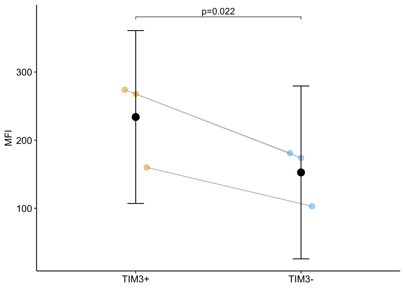
16.9.6 By modeling non-independence, the researchers gained free power
lm1 <- lm(nr4a1 ~ genotype, data = fig2c)
lm1_emm <- emmeans(lm1, specs = "genotype")
lm1_pairs <- contrast(lm1_emm, method = "revpairwise") |>
  summary(infer = TRUE)

# combine with random intercept and compare
model_table <- rbind(lmm.ri_pairs, lm1_pairs)
model_table |>
  kable(digits = c(1, 2, 2, 1, 2, 2, 2, 3)) |>
  kable_styling() |>
  pack_rows("lmm.ri:  random intercept model", 1, 1) |>
pack_rows("lm1: linear model", 2, 2)| contrast | estimate | SE | df | lower.CL | upper.CL | t.ratio | p.value |
|---|---|---|---|---|---|---|---|
| lmm.ri: random intercept model | |||||||
| (TIM3-) - (TIM3+) | -81.33 | 12.17 | 2 | -133.70 | -28.97 | -6.68 | 0.022 |
| lm1: linear model | |||||||
| (TIM3-) - (TIM3+) | -81.33 | 44.64 | 4 | -205.28 | 42.61 | -1.82 | 0.143 |
Notes
- The p-value for the linear model is 0.1426 while that of the random intercept model is 0.0217. Increased power will generally be the case with experimental bench biology data.
- More specifically, compared to the linear model, the random intercept model has increased precision of the effect estimate (a smaller SE) BUT also decreased degrees of freedom (df). The increased precision will always be the case if the correlated error is positive.
- Because of the increased precision but decreased df, there is a trade-off for inference using the linear mixed model (or classical equivalents) – increased precision increases power but decreased df decreases power. With even modest sample size (\(\sim 5\)), the increased precision will overwhelm the decreased df and power will increase. Here there is increased power even with n = 3.
16.9.7 Better Know the linear mixed model
Intraclass correlation
VarCorr(lmm.ri) Groups Name Std.Dev.
experiment_id (Intercept) 52.602
Residual 14.905 lmm.ri_vc <- VarCorr(lmm.ri) |>
data.frame() |>
data.table()
among_var <- lmm.ri_vc[1, vcov]
within_var <- lmm.ri_vc[2, vcov]
icc <- among_var/(among_var + within_var)
icc[1] 0.925676116.10 Example 3: RCBD with > 2 groups (classical equivalent: repeated measures ANOVA)
Source Figure: Fig 2C upper right (NR4A1)
Response variable: NR4A1 expression measured as MFI (mean flourescence intensity)
Treatment: CAR PD-1hi TIM3hi TILs, CAR PD-1hi TIM3lo TILs (so differ in density of TIM3 receptors)
Experimental Design: Randomized Complete Block Design (RCBD). Three preparations (experiments). Experiment is the block.
Background: CAR-T are T cells expressing chimeric antigen receptors and target/kill solid tumor cells. TILs are tumor infiltrating lymphocytes. NR are nuclear receptors that function as transcription factors. PD-1 and TIM3 are inhibitory receptors. CAR PD-1hi TIM3hi TILs are “highly exhausted”, CAR PD-1hi TIM3lo TILs are “antigen-specific memory precursor”
16.10.1 lmm.ri – random intercept model
lmm.ri <- lmer(nr4a1 ~ genotype + (1 | experiment_id), data = fig2c_r)
lmm.ri_emm <- emmeans(lmm.ri, specs = "genotype")
lmm.ri_pairs <- contrast(lmm.ri_emm, method = "revpairwise", adjust = "none") |>
  summary(infer = TRUE)
lmm.ri_pairs
contrast estimate SE df lower.CL upper.CL t.ratio p.value
(PD1+TIM3-) - (PD1+TIM3+) -69.8 11.7 4 -102.2 -37.3 -5.966 0.0040
(PD1-TIM3-) - (PD1+TIM3+) -82.8 11.7 4 -115.3 -50.3 -7.081 0.0021
(PD1-TIM3-) - (PD1+TIM3-) -13.0 11.7 4 -45.5 19.4 -1.115 0.3275
Degrees-of-freedom method: kenward-roger
Confidence level used: 0.95 16.10.3 rmaov.mul – repeated measures ANOVA (RM-ANOVA), multivariate model
rmaov.mul <- aov_4(nr4a1 ~ genotype + (genotype | experiment_id), data = fig2c_r)
rmaov.mul_emm <- emmeans(rmaov.mul, specs = "genotype")
rmaov.mul_pairs <- contrast(rmaov.mul_emm, method = "revpairwise", adjust = "none") |>
  summary(infer = TRUE)
rmaov.mul_pairs
contrast estimate SE df lower.CL upper.CL t.ratio p.value
PD1.TIM3..1 - PD1.TIM3. -69.8 9.44 2 -110.4 -29.1 -7.390 0.0178
PD1.TIM3..2 - PD1.TIM3. -82.8 15.70 2 -150.4 -15.2 -5.273 0.0341
PD1.TIM3..2 - PD1.TIM3..1 -13.0 8.63 2 -50.2 24.1 -1.510 0.2701
Confidence level used: 0.95 16.10.4 rmaov.uni – repeated measures ANOVA (RM-ANOVA), univariate model
rmaov.uni <- aov_4(nr4a1 ~ genotype + (genotype | experiment_id),
              data = fig2c_r,
              include_aov = TRUE)
aov1_emm <- emmeans(rmaov.uni,
                    specs = "genotype",
                    model = "univariate")
aov1_pairs <- contrast(aov1_emm,
                       method = "revpairwise",
                       adjust = "none") |>
  summary(infer = TRUE)
aov1_pairs
contrast estimate SE df lower.CL upper.CL t.ratio p.value
PD1.TIM3..1 - PD1.TIM3. -69.8 11.7 4 -102.2 -37.3 -5.966 0.0040
PD1.TIM3..2 - PD1.TIM3. -82.8 11.7 4 -115.3 -50.3 -7.081 0.0021
PD1.TIM3..2 - PD1.TIM3..1 -13.0 11.7 4 -45.5 19.4 -1.115 0.3275
Confidence level used: 0.95 16.10.5 pptt – pairwise paired t-test
ppttm <- pptt(nr4a1 ~ genotype + (1 | experiment_id), data = fig2c_r)
print(ppttm)
contrast estimate SE df lower.CL upper.CL
<char> <num> <num> <num> <num> <num>
1: PD1+TIM3- - PD1+TIM3+ -69.76667 9.440398 2 -110.38542 -29.14791
2: PD1-TIM3- - PD1+TIM3+ -82.80000 15.702654 2 -150.36307 -15.23693
3: PD1-TIM3- - PD1+TIM3- -13.03333 8.631403 2 -50.17126 24.10459
t.ratio p.value
<num> <num>
1: -7.390225 0.01782184
2: -5.272994 0.03413460
3: -1.509990 0.2701246916.10.6 Notes on the models
- lmm.ce fails.
- rmaov.mul and ppttm are equivalent. This is generally true if there are no missing data (genotype:experiment_id combinations). Both rmaov.mul and ppttm require balance but ppttm is a pairwise procedure while rmaov.mul analyzes all treatment levels simultaneously. Consequently ppttm will exclude fewer measures and will have slightly more power than rmaov.mul.
- rmaov.mul and lmm.ri are not equivalent and this is generally true.
- rmaov.uni and lmm.ri are equivalent and this is generally true if there are no missing data.
- The lmm equivalent of rmaov.mul is lmm.ris (random intercept and slopte model) but this model cannot be fit without replication with genotype:experiment_id combinations.
- One reasonable conclusion of item 4 is that rmaov.mul effectively overfits the data and we should use rmaov.uni/lmm.ri as the model of choice. The simulation under RCBD above argues against this. Instead, rmaov.mul/lmm.ris is preferred (although lmm.ris cannot be fit without replication)
- Item 5 raises the question, why bother with random intercept model in a RCBD? The random intercept model (lmm.ri) should be used if there are missing treatment:block combinations or if there are covariates or if the response should be modeled with a non-Normal distribution (distributions for counts, proportions, amounts) using a generalized linear model (glm).
16.10.7 Plot the model
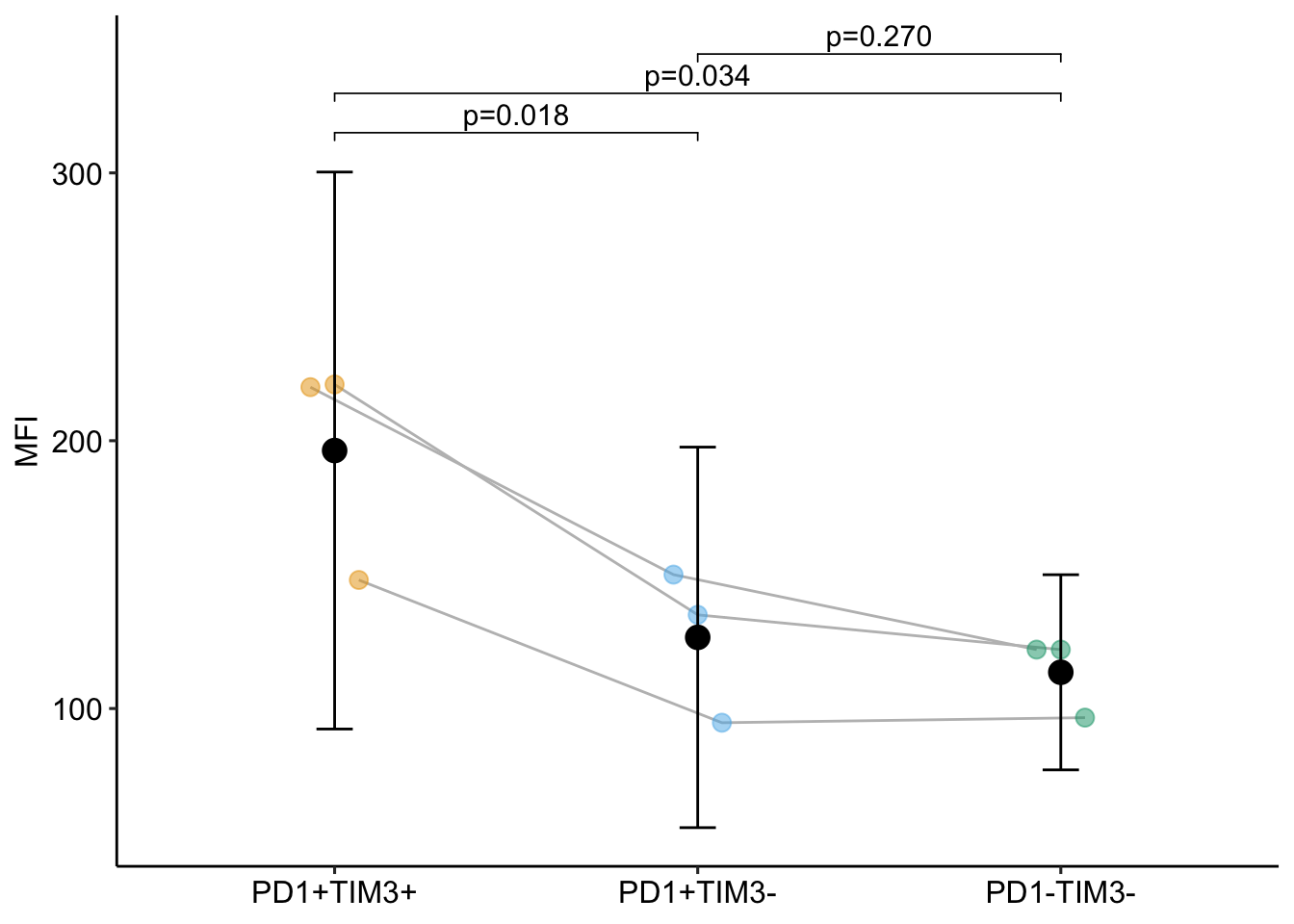
Notes
- The blocks are connected by the gray lines
- The modeled SE of the treatment means are large relative to the spread of the treatment replicates. The modeled SE of the treatment means are not a good guide to differences among the treatments in a model with random factors if the sample size (number of blocks) is small.
16.10.8 By modeling non-independence, the researchers gained free power
lm1 <- lm(nr4a1 ~ genotype, data = fig2c_r)
lm1_emm <- emmeans(lm1, specs = "genotype")
lm1_pairs <- contrast(lm1_emm, method = "revpairwise", adjust = "none") |>
  summary(infer = TRUE)

# replace contrast labels in rmaov.mul_pairs with readable labels
rmaov.mul_pairs$ contrast <- lm1_pairs$contrast
# combine with random intercept and compare
model_table <- rbind(rmaov.mul_pairs, lm1_pairs)
model_table |>
  kable(digits = c(1, 2, 2, 1, 2, 2, 2, 3)) |>
  kable_styling() |>
  pack_rows("lmm.ri:  multivariate RM-ANOVA model", 1, 3) |>
pack_rows("lm1: linear model", 4, 6)| contrast | estimate | SE | df | lower.CL | upper.CL | t.ratio | p.value |
|---|---|---|---|---|---|---|---|
| lmm.ri: multivariate RM-ANOVA model | |||||||
| (PD1+TIM3-) - (PD1+TIM3+) | -69.77 | 9.44 | 2 | -110.39 | -29.15 | -7.39 | 0.018 |
| (PD1-TIM3-) - (PD1+TIM3+) | -82.80 | 15.70 | 2 | -150.36 | -15.24 | -5.27 | 0.034 |
| (PD1-TIM3-) - (PD1+TIM3-) | -13.03 | 8.63 | 2 | -50.17 | 24.10 | -1.51 | 0.270 |
| lm1: linear model | |||||||
| (PD1+TIM3-) - (PD1+TIM3+) | -69.77 | 24.88 | 6 | -130.64 | -8.89 | -2.80 | 0.031 |
| (PD1-TIM3-) - (PD1+TIM3+) | -82.80 | 24.88 | 6 | -143.68 | -21.92 | -3.33 | 0.016 |
| (PD1-TIM3-) - (PD1+TIM3-) | -13.03 | 24.88 | 6 | -73.91 | 47.84 | -0.52 | 0.619 |
Notes
- Only two of the three p-values are smaller for the RM-ANOVA model. Increased power will generally be the case with experimental bench biology data.
- More specifically, compared to the linear model, the RM-ANOVA model has increased precision of the effect estimate (a smaller SE) BUT also decreased degrees of freedom (df). The increased precision will always be the case if the correlated error is positive.
- Because of the increased precision but decreased df, there is a trade-off for inference using the linear mixed model (or classical equivalents) – increased precision increases power but decreased df decreases power. With even modest sample size (\(\sim 5\)), the increased precision will overwhelm the decreased df and power will increase. Here there is increased power in two of the three contrasts even with n = 3.
16.11 Example 4 – RCBD with two factors (fig5c)
The data for Example 4 are from Figure 5c, which is a 2 x 2 factorial design with factors \(\texttt{treatment}\) and \(\texttt{activity}\). While there is no replication of \(\texttt{treatment:activity}\) combinations within a block, there are two measures of each factor level within a block and these two measures can act as a kind of replicate. Consequently, we can fit interaction intercept models.
Transcriptomic profiling of skeletal muscle adaptations to exercise and inactivity
Source figure: Fig. 5c
Source data: Source Data Fig. 5
16.11.1 Understand the data
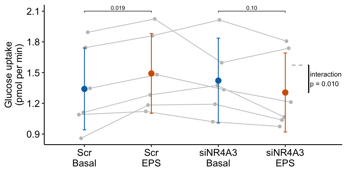
The data for Example 4 are from Figure 5c. Six muscle source cells were used to start six independent cultures. Cells from each culture were treated with either a negative control (“Scr”) or a siRNA (“siNR4A3”) that “silences” expression of the NR4A3 gene product by cleaving the mRNA. Glucose uptake in the two cell types was measured at rest (“Basal”) and during electrical pulse stimulation (“EPS”).
The design is a \(2 \times 2\) Randomized complete block with no subsampling. There are two factors each with two levels: \(\texttt{treatment}\) (“Scr”, “siNR4A3”) and \(\texttt{activity}\) (“Basal”, “EPS”). Each source cell is a block. All four treatment combinations were measured once per block.
16.11.2 Examine the data
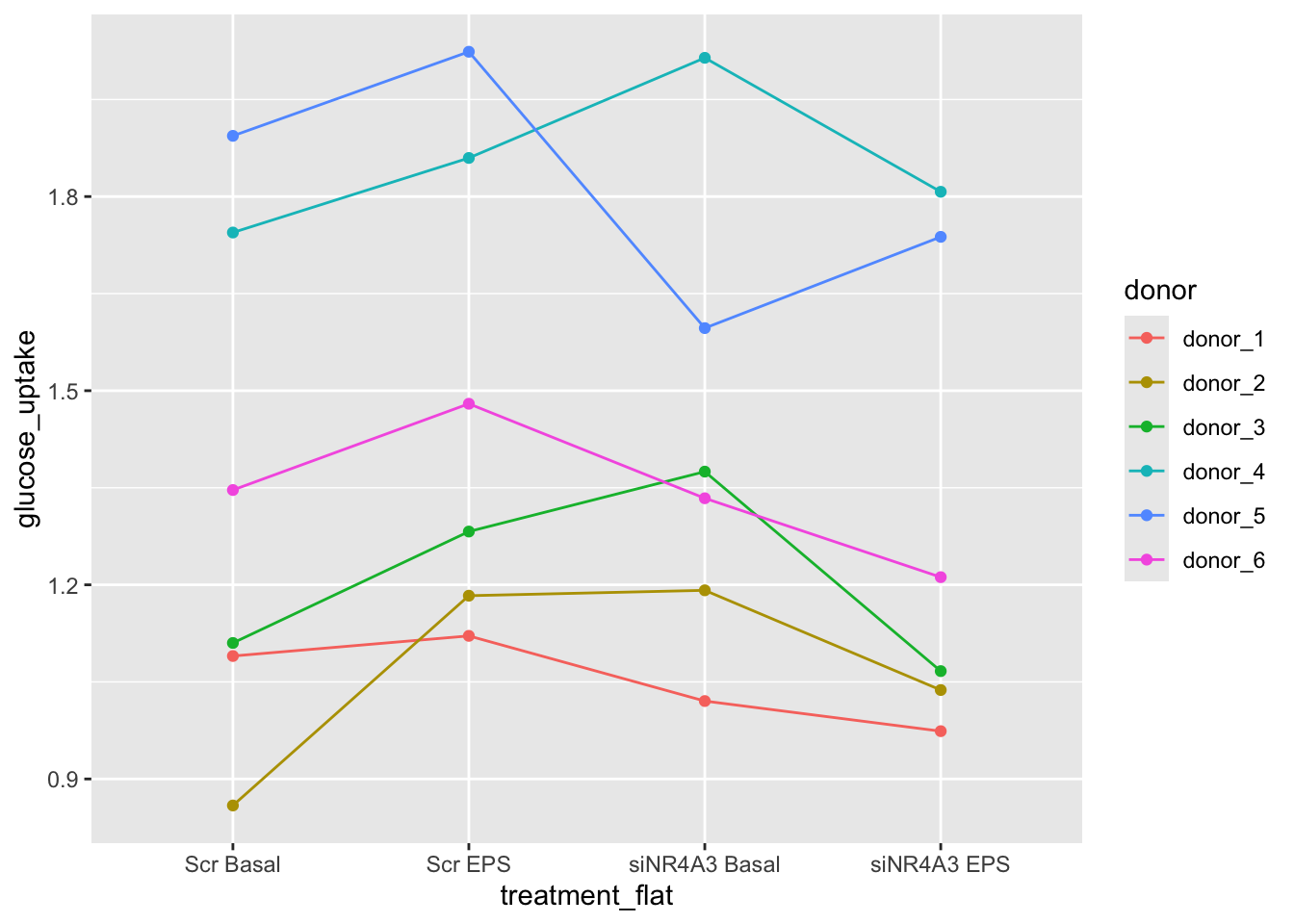
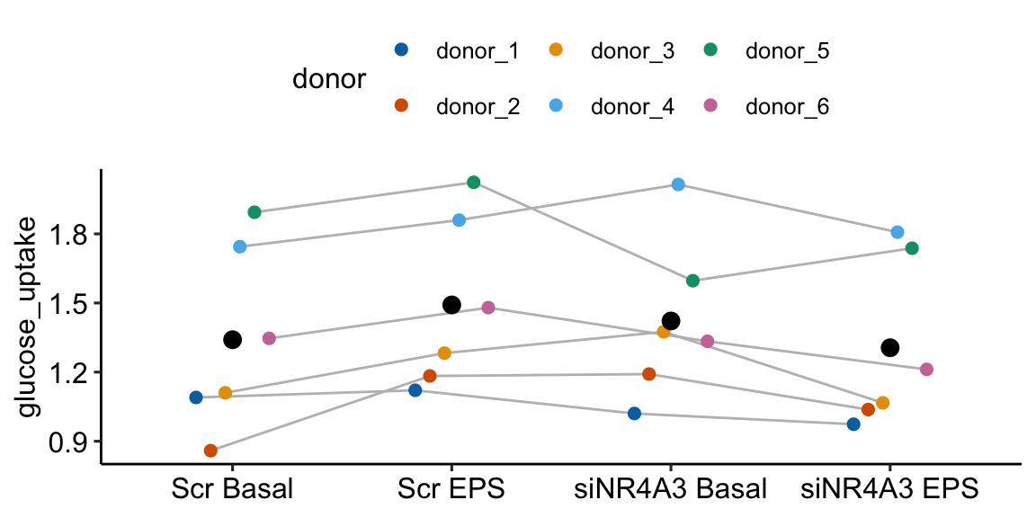
The plot shows a strong donor effect.
16.11.3 Model fit and inference
fig5c.ri <- lmer(glucose_uptake ~ treatment * activity +
                   (1 | donor),
                 data = fig5c)

fig5c.rii <- lmer(glucose_uptake ~ treatment * activity +
                   (1 | donor) +
                   (1 | donor:treatment) +
                   (1 | donor:activity),
                 data = fig5c)
# boundary warning

fig5c.rii2 <- lmer(glucose_uptake ~ treatment * activity +
                   (1 | donor) +
                   (1 | donor:treatment),
                 data = fig5c)

fig5c.rii3 <- lmer(glucose_uptake ~ treatment * activity +
                   (1 | donor) +
                   (1 | donor:activity),
                 data = fig5c)
# boundary warning

fig5c.ce <- lme(glucose_uptake ~ treatment * activity,
                 random =  ~ 1 | donor,
                 correlation = corCompSymm(form = ~ 1 | donor),
                 weights = varIdent(form = ~ 1|treatment_flat),
                 data = fig5c)

fig5c.rmaov <- aov_4(glucose_uptake ~ treatment * activity +
                   (treatment * activity | donor),
                 data = fig5c)

# check AIC
AIC(fig5c.ri, fig5c.rii2, fig5c.ce)
df AIC
fig5c.ri 6 8.153813
fig5c.rii2 7 8.052676
fig5c.ce 10 9.885960# check VarCorr model c
VarCorr(fig5c.rii2) # fine Groups Name Std.Dev.
donor:treatment (Intercept) 0.089519
donor (Intercept) 0.352097
Residual 0.090685# report fig5c_lmm2.rii (based on AIC and VarCorr check)
fig5c_m1 <- fig5c.ceThe boundary warnings indicate a variance component with no estimated variance, so these are excluded. There is trivial difference in AIC between fig5c_lmm.ri and fig5c_lmm2.rii and fig5c_ce <2 units from these. I recommend choosing to report the most maximal model (fig5c_ce or fig5c_rmaov.mul).
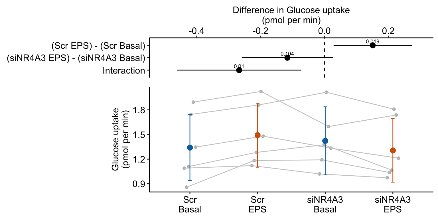
fig5c_m1_emm <- emmeans(fig5c_m1, specs = c("treatment", "activity"))| treatment | activity | emmean | SE | df | lower.CL | upper.CL |
|---|---|---|---|---|---|---|
| Scr | Basal | 1.34 | 0.155 | 5 | 0.94 | 1.74 |
| siNR4A3 | Basal | 1.42 | 0.161 | 5 | 1.01 | 1.84 |
| Scr | EPS | 1.49 | 0.152 | 5 | 1.10 | 1.88 |
| siNR4A3 | EPS | 1.31 | 0.150 | 5 | 0.92 | 1.69 |
# fig5c_emm # print in console to get row numbers
# set the mean as the row number from the emmeans table
scr_basal <- c(1,0,0,0)
siNR4A3_basal <- c(0,1,0,0)
scr_eps <- c(0,0,1,0)
siNR4A3_eps <- c(0,0,0,1)

fig5c_m1_planned <- contrast(fig5c_m1_emm,
                       method = list(
                         "(Scr EPS) - (Scr Basal)" = c(scr_eps - scr_basal),
                         "(siNR4A3 EPS) - (siNR4A3 Basal)" = c(siNR4A3_eps - siNR4A3_basal),
                         "Interaction" = c(siNR4A3_eps - siNR4A3_basal) -
                           c(scr_eps - scr_basal)

                       ),
                       adjust = "none"
) |>
summary(infer = TRUE)| contrast | estimate | SE | df | lower.CL | upper.CL | t.ratio | p.value |
|---|---|---|---|---|---|---|---|
| (Scr EPS) - (Scr Basal) | 0.15 | 0.057 | 15 | 0.03 | 0.27 | 2.63 | 0.019 |
| (siNR4A3 EPS) - (siNR4A3 Basal) | -0.12 | 0.067 | 15 | -0.26 | 0.03 | -1.73 | 0.104 |
| Interaction | -0.27 | 0.091 | 15 | -0.46 | -0.07 | -2.93 | 0.010 |
16.11.3.1 Plot the model
16.11.3.2 Alternaplot the model
Notes
- Many researchers might look at the wide confidence intervals relative to the short distance between the means and think “no effect”. The confidence intervals are correct, they simply are not meant to be tools for inferring anything about differences in means. This is one of many reasons why plots of means and error bars can be misleading for inference, despite the ubiquity of their use for communicating results. And, its why I prefer the effects-and-response plots, which explicitly communicate correct inference about effects.
16.11.4 Why we care about modeling the blocks in fig5c
Figure 16.9 shows the modeled means of the four treatment combinations and the individual values colored by donor. It is pretty easy to see that the glucose uptake values for donors 4 and 5 are well above the mean for all four treatments. And, the values for donors 1, 2, and 3 are well below the mean for all four treatments. The values for donor 6 are near the mean for all four treatments.
Let’s compare the effects estimated by the linear mixed model fig5c_m1 with a linear model that ignores donor.
fig5c_m2 <- lm(glucose_uptake ~ treatment * activity,
           data = fig5c)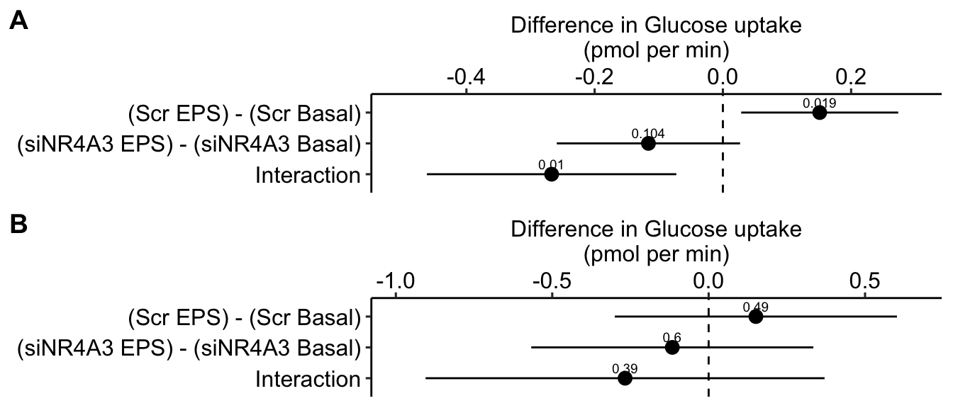
Figure 16.10 A is a plot of the effects from the linear mixed model that models the correlated error due to donor. Figure 16.10 B is a plot of the effects from the fixed effect model that ignores the correlated error due to donor. Adding \(\texttt{donor}\) as a factor to the linear model increases the precision of the estimate of the treatment effects by eliminating the among-donor component of variance from the error variance.
16.12 Example 5 – GRCBD Experiments with replication (exp1g)
This example is from a design with batches (independent experiments) that contain all treatment levels of a single factor and replication. These data were used to introduce linear mixed models in Example 1. The design of the experiment is \(2 \times 2\) factorial. Example 1 flattened the analysis to simplify explanation of random intercepts and random slopes. Here, the data are analyzed with a factorial model.
A GPR174–CCL21 module imparts sexual dimorphism to humoral immunity
Source figure: Fig. 1g
Source data: Source Data Fig. 1
16.12.1 Understand the data
The researchers in this paper are interested in discovering mechanisms causing the lower antibody-mediated immune response in males relative to females. The data in Fig. 1 are from a set of experiments on mice to investigate how the G-protein coupled receptor protein GPR174 regulates formation of the B-cell germinal center in secondary lymph tissue. GPR174 is a X-linked gene.
Response variable \(\texttt{gc}\) – germinal center size (%). The units are the percent of cells expressing germinal center markers.
Factor 1 – \(\texttt{sex}\) (“M”, “F”). Male (“M”) is the reference level.
Factor 2 – \(\texttt{chromosome}\) (“Gpr174+”, “Gpr174-”). “Gpr174-” is a GPR174 knockout. The wildtype (“Gpr174+”) condition is the reference level.
Design – \(2 \times 2\), that is, two crossed factors each with two levels. This results in four groups, each with a unique combination of the levels from each factor. “M Gpr174+” is the control. “M Gpr174+” is the knockout genotype in males (“knockout added”). “F Gpr174+” is the wildtype female (“X chromosome added”). “F Gpr174-” is the knockout female (“knockout and X chromosome added”.
16.12.2 Examine the data
ggplot(data = exp1g,
       aes(x = treatment,
           y = gc,
           color = experiment_id)) +
  geom_point(position = position_dodge(0.4))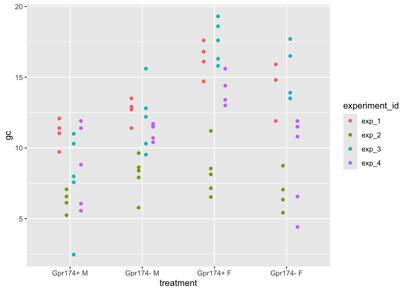
16.12.3 Fit the model
# three slope parameters
exp1g_m1a <- lmer(gc ~ genotype * sex +
                   (genotype * sex | experiment_id),
                 data = exp1g)
boundary (singular) fit: see help('isSingular')VarCorr(exp1g_m1a) # looks fine Groups Name Std.Dev. Corr
experiment_id (Intercept) 1.77088
genotypeGpr174- 0.96193 -0.023
sexF 2.90154 0.459 0.878
genotypeGpr174-:sexF 1.33170 -0.314 -0.625 -0.706
Residual 1.93155 # one slope parameter but capturing all treatment combinations
exp1g_m1b <- lmer(gc ~ genotype * sex +
(treatment | experiment_id),
data = exp1g)
# intercept interactions
exp1g_m1c <- lmer(gc ~ genotype * sex +
(1 | experiment_id) +
(1 | experiment_id:genotype) +
(1 | experiment_id:sex) +
(1 | experiment_id:genotype:sex),
data = exp1g)boundary (singular) fit: see help('isSingular')VarCorr(exp1g_m1c) # id:genotype is low Groups Name Std.Dev.
experiment_id:genotype:sex (Intercept) 0.4046670
experiment_id:sex (Intercept) 1.6927499
experiment_id:genotype (Intercept) 0.0001216
experiment_id (Intercept) 2.5487069
Residual 1.9792428# drop id:genotype which has low variance
exp1g_m1d <- lmer(gc ~ genotype * sex +
(1 | experiment_id) +
(1 | experiment_id:sex) +
(1 | experiment_id:sex:genotype),
data = exp1g)
AIC(exp1g_m1a, exp1g_m1b, exp1g_m1c, exp1g_m1d) df AIC
exp1g_m1a 15 344.1579
exp1g_m1b 15 344.1529
exp1g_m1c 9 337.7602
exp1g_m1d 8 335.7602# go with exp1g_m1d.
exp1g_m1 <- exp1g_m1d16.12.4 Inference from the model
exp1g_m1_coef <- coef(summary(exp1g_m1))exp1g_m1_coef Estimate Std. Error df t value Pr(>|t|)
(Intercept) 8.435718 1.612602 4.638595 5.231123 0.004202015
genotypeGpr174- 2.568365 0.712122 5.760582 3.606637 0.012094327
sexF 5.583860 1.397388 4.024010 3.995927 0.015995349
genotypeGpr174-:sexF -5.304752 1.013552 5.918159 -5.233823 0.002033657# order of factors reversed in specs because I want sex to be
# main x-axis variable in plot
exp1g_m1_emm <- emmeans(exp1g_m1, specs = c("sex", "genotype"))# exp1g_m1_emm # print in console to get row numbers
# set the mean as the row number from the emmeans table
wt_m <- c(1,0,0,0)
wt_f <- c(0,1,0,0)
ko_m <- c(0,0,1,0)
ko_f <- c(0,0,0,1)
# simple effects within males and females + interaction
# 1. (ko_m - wt_m)
# 2. (ko_f - wt_f)
exp1g_contrasts <- list(
"(Gpr174- M) - (Gpr174+ M)" = c(ko_m - wt_m),
"(Gpr174- F) - (Gpr174+ F)" = c(ko_f - wt_f),
"Interaction" = c(ko_f - wt_f) -
c(ko_m - wt_m)
)
exp1g_m1_planned <- contrast(exp1g_m1_emm,
method = exp1g_contrasts,
adjust = "none"
) |>
summary(infer = TRUE)| contrast | estimate | SE | df | lower.CL | upper.CL | t.ratio | p.value |
|---|---|---|---|---|---|---|---|
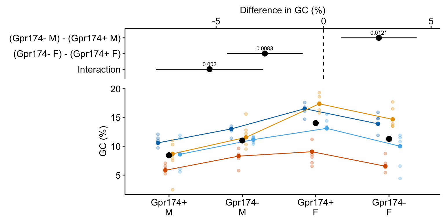
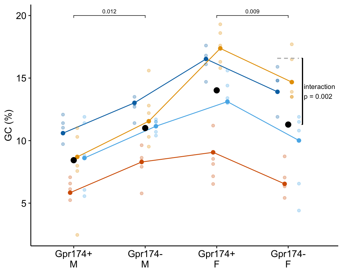
| (Gpr174- M) - (Gpr174+ M) | 2.57 | 0.714 | 5.784 | 0.81 | 4.33 | 3.60 | 0.012 |
| (Gpr174- F) - (Gpr174+ F) | -2.74 | 0.722 | 6.100 | -4.50 | -0.98 | -3.79 | 0.009 |
| Interaction | -5.30 | 1.016 | 5.942 | -7.80 | -2.81 | -5.22 | 0.002 |
Notes
- The direction of the estimated effect is opposite in males and females
16.12.5 Plot the model
16.12.6 Alternaplot the model
16.12.7 Understanding the alternative models
exp1g_m1a <- lmer(gc ~ genotype * sex +
                   (genotype * sex | experiment_id),
                 data = exp1g)
boundary (singular) fit: see help('isSingular')exp1g_m1b <- lmer(gc ~ genotype * sex +
(treatment | experiment_id),
data = exp1g)
exp1g_m1c <- lmer(gc ~ genotype * sex +
(1 | experiment_id) +
(1 | experiment_id:genotype) +
(1 | experiment_id:sex) +
(1 | experiment_id:genotype:sex),
data = exp1g)boundary (singular) fit: see help('isSingular')exp1g_m1d <- lmer(gc ~ genotype * sex +
(1 | experiment_id) +
(1 | experiment_id:sex) +
(1 | experiment_id:genotype:sex),
data = exp1g)Notes
- All four models model the same fixed effects. The models differ only in how they model the random effects.
- Model
exp1g_m1afits one random intercept, two random slopes, and one random interaction.
- \(\gamma_{0j}\) – a random intercept modeling batch effects of \(\texttt{experiment\_id}\) on the intercept
- \(\gamma_{1j}\) – a random slope modeling the effect of the non-reference level of “Gpr174-” on the batch effect of \(\texttt{experiment\_id}\). This is a \(\texttt{experiment\_id} \times \texttt{genotype}\) interaction.
- \(\gamma_{2j}\) – a random slope modeling the effect of “F” (female) on the batch effect of \(\texttt{experiment\_id}\). This is a \(\texttt{experiment\_id} \times \texttt{sex}\) interaction.
- \(\gamma_{3j}\) – a random slope modeling the effect of the interaction effect of “Gpr174-” and “F” on the batch effect of \(\texttt{experiment\_id}\). This is a \(\texttt{experiment\_id} \times \texttt{sex} \times \texttt{genotype}\) interaction.
- Model
exp1g_m1bfits one random intercept and three random slopes
- \(\gamma_{0j}\) – a random intercept modeling batch effects of \(\texttt{experiment\_id}\) on the intercept. This is modeling the same thing as \(\gamma_{0j}\) in Model
exp1g_m1a. - \(\gamma_{1j}\) – a random slope modeling the effect of “Gpr174- M” on the batch effect of \(\texttt{experiment\_id}\). This is modeling the same thing as \(\gamma_{1j}\) in Model
exp1g_m1a. - \(\gamma_{2j}\) – a random slope modeling the effect of “Gpr174+ F” on the batch effect of \(\texttt{experiment\_id}\). This is modeling the same thing as \(\gamma_{2j}\) in Model
exp1g_m1a. - \(\gamma_{3j}\) – a random slope modeling the effect of “M Gpr174- F” on the batch effect of \(\texttt{experiment\_id}\). This is modeling the added variance accounted for by the random interaction \(\gamma_{2j}\) in Model
exp1g_m1abut in a different way.
- Model
exp1g_m1cfits four random intercepts
- \(\gamma_{0j}\) – a random intercept modeling batch effects of \(\texttt{experiment\_id}\) on the intercept. This is modeling the same thing as \(\gamma_{0j}\) in Model
exp1g_m1a. - \(\gamma_{0jk}\) – a random intercept modeling the effects of the combination of \(\texttt{experiment\_id}\) and \(\texttt{genotype}\). This is very similar to the variance modeled by \(\gamma_{1j}\) in Model
exp1g_m1aexcept the draws from \(\gamma_{0jk}\) are independent (uncorrelated) of draws from the other random intercepts. - \(\gamma_{0jl}\) – a random intercept modeling the effects of the combination of \(\texttt{experiment\_id}\) and \(\texttt{sex}\). This is very similar to the variance modeled by \(\gamma_{2j}\) in Model
exp1g_m1aexcept the draws from \(\gamma_{0jl}\) are independent (uncorrelated) of draws from the other random intercepts (review The correlation among random intercepts and slopes if this doesn’t make sense). - \(\gamma_{0jkl}\) – a random intercept modeling the effects of the combination of \(\texttt{experiment\_id}\), \(\texttt{genotype}\) and \(\texttt{sex}\). This is very similar to the variance modeled by \(\gamma_{3j}\) in Model
exp1g_m1aexcept the draws from \(\gamma_{0jkl}\) are independent (uncorrelated) of draws from the other random intercepts.
- Model
exp1g_m1dfits the same random intercepts as Modelexp1g_m1cbut excludes \(\gamma_{0jl}\) (the random intercept for the experiment_id by genotyp combination. This was excluded because of the low variance of this component in the fit model.
16.12.8 The VarCorr matrix of models exp1g_m1a and exp1g_m1b
The random effect similarity of models exp1g_m1a and exp1g_m1b can be seen in the estimated variance components and correlations among the random effects.
| exp1g_m1a | ||||
| (Intercept) | 1.7709 | |||
| genotypeGpr174- | -0.0232 | 0.9619 | ||
| sexF | 0.4589 | 0.8776 | 2.9015 | |
| genotypeGpr174-:sexF | -0.3137 | -0.6247 | -0.7056 | 1.3317 |
| exp1g_m1b | ||||
| (Intercept) | 1.7711 | |||
| treatmentGpr174- M | -0.0250 | 0.9641 | ||
| treatmentGpr174+ F | 0.4585 | 0.8761 | 2.9024 | |
| treatmentGpr174- F | 0.2999 | 0.8793 | 0.9384 | 2.9909 |
16.12.9 The linear mixed model has more precision and power than the fixed effect model of batch means
# means pooling model
exp1g_m2 <- lm(gc ~ sex * genotype,
data = exp1g_means)| contrast | estimate | SE | df | lower.CL | upper.CL | t.ratio | p.value |
|---|---|---|---|---|---|---|---|
| exp1g_m1 (lmm) | |||||||
| (Gpr174- M) - (Gpr174+ M) | 2.57 | 0.714 | 5.8 | 0.81 | 4.33 | 3.60 | 0.012 |
| (Gpr174- F) - (Gpr174+ F) | -2.74 | 0.722 | 6.1 | -4.50 | -0.98 | -3.79 | 0.009 |
| Interaction | -5.30 | 1.016 | 5.9 | -7.80 | -2.81 | -5.22 | 0.002 |
| exp1g_m2 (lm means pooling) | |||||||
| (Gpr174- M) - (Gpr174+ M) | 2.50 | 2.257 | 12.0 | -2.41 | 7.42 | 1.11 | 0.289 |
| (Gpr174- F) - (Gpr174+ F) | -2.73 | 2.257 | 12.0 | -7.65 | 2.18 | -1.21 | 0.249 |
| Interaction | -5.24 | 3.192 | 12.0 | -12.20 | 1.72 | -1.64 | 0.127 |
Notes
- A fixed effects model fit to batch-means pooled data is strongly conservative and will result in less discovery.
- Means pooling does not make the data independent in a randomized complete block design. A linear mixed model of batch-means pooled data is a mixed-effect ANOVA (Next section. Also see Section @ref(issues-exp4d) in the Issues chapter).
16.12.10 Fixed effect models and pseudoreplication
# complete pooling model
exp1g_m3 <- lm(gc ~ sex * genotype,
data = exp1g)| contrast | estimate | SE | df | lower.CL | upper.CL | t.ratio | p.value |
|---|---|---|---|---|---|---|---|
| exp1g_m1 (lmm) | |||||||
| (Gpr174- M) - (Gpr174+ M) | 2.57 | 0.714 | 5.8 | 0.81 | 4.33 | 3.60 | 0.012 |
| (Gpr174- F) - (Gpr174+ F) | -2.74 | 0.722 | 6.1 | -4.50 | -0.98 | -3.79 | 0.009 |
| Interaction | -5.30 | 1.016 | 5.9 | -7.80 | -2.81 | -5.22 | 0.002 |
| exp1g_m3 (lm complete pooling) | |||||||
| (Gpr174- M) - (Gpr174+ M) | 2.44 | 1.111 | 69.0 | 0.22 | 4.65 | 2.20 | 0.032 |
| (Gpr174- F) - (Gpr174+ F) | -2.53 | 1.125 | 69.0 | -4.77 | -0.28 | -2.25 | 0.028 |
| Interaction | -4.97 | 1.581 | 69.0 | -8.12 | -1.81 | -3.14 | 0.002 |
Notes
- Complete pooling is strongly anti-conservative and will result in increased false discovery. Complete pooling is a type of pseudoreplication – the subsamples have been analyzed as if they are independent replicates. Subsamples are not independent.
- For the Experiment 1g data, the 95% confidence intervals are wider and the p-values are larger in the complete pool model
exp1g_m3compared to the linear mixed modelexp1g_m1. This is an unusual result.
16.12.11 Mixed-effect ANOVA
exp1g_m1_aov <- aov_4(gc ~ sex * genotype +
                  (sex * genotype | experiment_id),
                data = exp1g)
Warning: More than one observation per design cell, aggregating data using `fun_aggregate = mean`.
To turn off this warning, pass `fun_aggregate = mean` explicitly.Notes
- The formula has the same format as that in Example 3 for repeated measures ANOVA on RCB designs with no subsampling. In biology, this is often called a mixed effect ANOVA with two fixed factors and one random factor.
- The data are aggregated prior to fitting the model – this means the subsamples are averaged within each batch by treatment combination.
- The mixed-effect ANOVA is equivalent to the linear mixed model
exp1g_m1cif there are the same number of replicates in each treatment combination and the same number of subsamples in all treatment by \(\texttt{experiment\_id}\) combinations. The design is not balanced in this example.
| contrast | estimate | SE | df | lower.CL | upper.CL | t.ratio | p.value |
|---|---|---|---|---|---|---|---|
| exp1g_m1_aov (mixed ANOVA) | |||||||
| (Gpr174- M) - (Gpr174+ M) | 2.50 | 0.599 | 3.000 | 0.60 | 4.41 | 4.18 | 0.025 |
| (Gpr174- F) - (Gpr174+ F) | -2.73 | 0.808 | 3.000 | -5.30 | -0.16 | -3.39 | 0.043 |
| Interaction | -5.24 | 1.087 | 3.000 | -8.70 | -1.78 | -4.82 | 0.017 |
| exp1g_m1_c (lmm equivalent of mixed ANOVA) | |||||||
| (Gpr174- M) - (Gpr174+ M) | 2.57 | 0.715 | 5.784 | 0.80 | 4.33 | 3.59 | 0.012 |
| (Gpr174- F) - (Gpr174+ F) | -2.74 | 0.724 | 6.100 | -4.50 | -0.97 | -3.78 | 0.009 |
| Interaction | -5.30 | 1.017 | 2.972 | -8.56 | -2.05 | -5.21 | 0.014 |
| exp1g_md (lmm with min AIC) | |||||||
| (Gpr174- M) - (Gpr174+ M) | 2.57 | 0.714 | 5.784 | 0.81 | 4.33 | 3.60 | 0.012 |
| (Gpr174- F) - (Gpr174+ F) | -2.74 | 0.722 | 6.100 | -4.50 | -0.98 | -3.79 | 0.009 |
| Interaction | -5.30 | 1.016 | 5.942 | -7.80 | -2.81 | -5.22 | 0.002 |
16.13 Example 6 Split Plot Design
Source: Diabetes relief in mice by glucose-sensing insulin-secreting human α-cells
Source figure: Figure 1f
16.13.1 Understand the data
The experiment for Fig. is a 3 x 2 factorial designed arranged as a split plot design. Donor cells are randomly assigned to one of three levels of the factor treatment (αGFP, αpm, αpm+HM). Within a donor, cells are divided into two levels of the factor glucose (low, high). In the language of Split Plot experiments, treatment is the Main Plot factor, because each replication is a unique donor. And, glucose is the Subplot factor, because both levels are within each Main plot. Note that in a split plot design, non-independence is only within a level of the Main Plot. If the design were blocked, a donor would be split between all combinations of treatment:glucose but here, a donor is only split among glucose within a treatment level (aGFP or aPM or aPM_HM).
Factor variables
- Factor 1 (Main plot):
treatment
- αGFP – the control
- αpm – PDX1 + MAFA.
- αpm+HM – αpm + HM.
- Factor 2 (Subplot)
glucose
- low – 3 mmol glucose
- high – 20 mmol glucose
Response variable: c-peptide (fmol per \(10^3\) cells per hour)
Biological Background
- Pdx1 and MafA are transcription factors that stimulate differentiation of pancreatic alpha cells into insulin-secreting beta cells.
- HM is a combination of human mesenchymal stem cells (MSCs) and human umbilical vein endothelial cells (HUVECs) and provide the appropriate environment for the alpha cells to produce insulin.
- c-peptide is a stretch of amino-acids in between the alpha and beta subunits of insulin in the pro-insulin protein. Within the secretory vesicle, the c-peptide is cleaved leaving the alpha and beta subunits to form the insulin protein. c-peptide and insulin are secreted 1:1 so measures of c-peptide are markers of insulin secretion.
data_from <- "Diabetes relief in mice by glucose-sensing insulin-secreting human α-cells"
file_name <- "41586_2019_942_MOESM7_ESM.xlsx"
file_path <- here(data_folder, data_from, file_name)

# IMPORTANT -- the numbers in the excel file have to be re-formatted
# to "general", otherwise, these are imported as dates
glucose_levels <- c("Low", "Hi")
fig1f_wide <- read_excel(file_path,
                         sheet = "Fig.1",
                         range = "C28:D43",
                         col_names = TRUE) %>%
  data.table()

fig1f_wide[, donor_id := paste0("donor_", .I)]
treatment_levels <- c("αGFP", "αPM", "αPM+HM")
fig1f_wide[, treatment := factor(rep(treatment_levels, each = 5),
           levels = treatment_levels)]

fig1f <- melt(fig1f_wide,
              id.vars = c("treatment", "donor_id"),
              measure.vars = glucose_levels,
              variable.name = "glucose",
              value.name = "c_peptide")
# View(fig1f)

fig1f[, .(N = .N), by = .(treatment, glucose)]
treatment glucose N
<fctr> <fctr> <int>
1: αGFP Low 5
2: αPM Low 5
3: αPM+HM Low 5
4: αGFP Hi 5
5: αPM Hi 5
6: αPM+HM Hi 516.13.2 lmm.sp linear mixed model for split plot design
lmm.sp <- lmer(c_peptide ~ treatment * glucose + (1 | donor_id), data = fig1f)
lmm.sp_emm <- emmeans(lmm.sp, specs = c("treatment", "glucose"))
lmm.sp_pairs <- contrast(lmm.sp_emm,
                         method = "revpairwise",
                         simple = "each",
                         combine = TRUE,
                         adjust = "none") |>
  summary(infer = TRUE)
rmaov.sp <- aov_4(c_peptide ~ treatment * glucose + (glucose | donor_id), data = fig1f)Contrasts set to contr.sum for the following variables: treatmentrmaov.sp_emm <- emmeans(rmaov.sp, specs = c("treatment", "glucose"))
rmaov.sp_pairs <- contrast(rmaov.sp_emm,
method = "revpairwise",
simple = "each",
combine = TRUE,
adjust = "none") |>
summary(infer = TRUE)pairs_dt <- rbind(lmm.sp_pairs, rmaov.sp_pairs)
pairs_dt |>
kable(digits = c(1,1,1,3,3,2,3,3,2,5), caption = "Planned contrasts from mixed ANOVA compared to lmm equivalent of mixed ANOVA and lowest AIC lmm.") |>
kable_styling() |>
pack_rows("lmm.sp lmm random intercept", 1, 9) |>
pack_rows("rmaov.sp RMANOVA for split plot", 10, 18)| glucose | treatment | contrast | estimate | SE | df | lower.CL | upper.CL | t.ratio | p.value |
|---|---|---|---|---|---|---|---|---|---|
| lmm.sp lmm random intercept | |||||||||
| Low | . | αPM - αGFP | 0.058 | 0.039 | 20.43 | -0.023 | 0.140 | 1.49 | 0.15251 |
| Low | . | (αPM+HM) - αGFP | 0.062 | 0.039 | 20.43 | -0.019 | 0.144 | 1.59 | 0.12643 |
| Low | . | (αPM+HM) - αPM | 0.004 | 0.039 | 20.43 | -0.077 | 0.086 | 0.11 | 0.91564 |
| Hi | . | αPM - αGFP | 0.127 | 0.039 | 20.43 | 0.046 | 0.209 | 3.25 | 0.00395 |
| Hi | . | (αPM+HM) - αGFP | 0.249 | 0.039 | 20.43 | 0.167 | 0.330 | 6.35 | 0.00000 |
| Hi | . | (αPM+HM) - αPM | 0.121 | 0.039 | 20.43 | 0.040 | 0.203 | 3.10 | 0.00555 |
| . | αGFP | Hi - Low | 0.017 | 0.030 | 12.00 | -0.048 | 0.082 | 0.56 | 0.58418 |
| . | αPM | Hi - Low | 0.086 | 0.030 | 12.00 | 0.021 | 0.151 | 2.87 | 0.01403 |
| . | αPM+HM | Hi - Low | 0.203 | 0.030 | 12.00 | 0.138 | 0.268 | 6.80 | 0.00002 |
| rmaov.sp RMANOVA for split plot | |||||||||
| Low | . | αPM - αGFP | 0.058 | 0.023 | 12.00 | 0.009 | 0.108 | 2.57 | 0.02477 |
| Low | . | (αPM+HM) - αGFP | 0.062 | 0.023 | 12.00 | 0.013 | 0.112 | 2.75 | 0.01759 |
| Low | . | (αPM+HM) - αPM | 0.004 | 0.023 | 12.00 | -0.045 | 0.054 | 0.19 | 0.85623 |
| Hi | . | αPM - αGFP | 0.127 | 0.051 | 12.00 | 0.017 | 0.237 | 2.52 | 0.02702 |
| Hi | . | (αPM+HM) - αGFP | 0.249 | 0.051 | 12.00 | 0.139 | 0.359 | 4.92 | 0.00035 |
| Hi | . | (αPM+HM) - αPM | 0.121 | 0.051 | 12.00 | 0.011 | 0.231 | 2.40 | 0.03334 |
| . | αGFP | Hi - Low | 0.017 | 0.030 | 12.00 | -0.048 | 0.082 | 0.56 | 0.58418 |
| . | αPM | Hi - Low | 0.086 | 0.030 | 12.00 | 0.021 | 0.151 | 2.87 | 0.01403 |
| . | αPM+HM | Hi - Low | 0.203 | 0.030 | 12.00 | 0.138 | 0.268 | 6.80 | 0.00002 |
Notes
- The design is balanced
- Within the treatment factor, where there are only two levels of the other factor, inference is the same between the lmm.sp and rmaov.sp.
- But, within the glucose factor, where there are three levels of the other factor, inference is different, because different SEs are computed for the Low vs. Hi contrasts. The rmaov.sp model is the more maximal model.
16.14 So, which model, and why? A simulation to help decide
16.14.1 Single factor RCBD models
With any design that creates non-independence, two linear mixed modeling strategies would be
- Fit the maximal model first, if the model fails or has boundary warning because of too little variance at some level, then fit the next most maximal model, and so on. For a RCBD with >2 groups, this order would be lmm.ce, lmm.ri, lm.fe (lmm.ri and lm.fe are equivalent if the design is balanced).
- Fit all linear mixed models and use a model selection method to choose the best model using a model selection method such as AIC.
I suggest a third strategy, which I prefer. This is,
- use simulation to compare the performance (Type I error and Power) of each model under differ combinations of the structure of the variances of the levels of the random factor. Use these results to guide the strategy
Here I use a simulation to measure the performance of the RCBD statistical models under four conditions of correlated error among the blocks between two treatment levels.
- High correlated error. There is heterogenous correlated error among the three pairs of treatments, with one high, one intermediate, and one low correlation
- Low correlated error. There is heterogenous correlated error among the three pairs of treatments, all with low correlation.
- Homogenous correlated error. There is high correlated errror among the three pairs of treatment, all with the same expected level
- There is no correlated error.
| Contrast | Cor Error | lm.crd | lm.fe | lmm.ce | rmaov.mul | rmaov.uni1x | ppttm |
|---|---|---|---|---|---|---|---|
| sim 1 - high correlated error | |||||||
| Tr1 - Cn | 0.302 | 0.050 | 0.108 | 0.070 | 0.058 | 0.108 | 0.058 |
| Tr2 - Cn | 0.411 | 0.024 | 0.082 | 0.064 | 0.046 | 0.082 | 0.046 |
| Tr2 - Tr1 | 0.657 | 0.000 | 0.006 | 0.076 | 0.072 | 0.006 | 0.072 |
| sim 2 - low correlated error | |||||||
| Tr1 - Cn | 0.175 | 0.052 | 0.088 | 0.076 | 0.068 | 0.088 | 0.068 |
| Tr2 - Cn | 0.158 | 0.684 | 0.736 | 0.698 | 0.652 | 0.736 | 0.652 |
| Tr2 - Tr1 | 0.229 | 0.726 | 0.788 | 0.876 | 0.826 | 0.788 | 0.826 |
| sim 3 - equal correlated error | |||||||
| Tr1 - Cn | 0.760 | 0.000 | 0.054 | 0.059 | 0.050 | 0.054 | 0.050 |
| Tr2 - Cn | 0.773 | 0.278 | 0.904 | 0.896 | 0.874 | 0.904 | 0.874 |
| Tr2 - Tr1 | 0.766 | 0.282 | 0.912 | 0.916 | 0.882 | 0.912 | 0.882 |
| sim 4 - zero correlated error | |||||||
| Tr1 - Cn | 0.045 | 0.054 | 0.058 | 0.070 | 0.046 | 0.058 | 0.046 |
| Tr2 - Cn | 0.020 | 0.272 | 0.268 | 0.282 | 0.232 | 0.268 | 0.232 |
| Tr2 - Tr1 | -0.021 | 0.310 | 0.292 | 0.302 | 0.262 | 0.292 | 0.262 |
The major result is
- The naive linear model, which doesn’t model the non-independence, can be slightly to extremely conservative. There is only good Type I error behavior only when there is something close to zero correlated error.
Results to inform our decision about which model for non-independence
- When there is zero correlated error, of the methods that model non-independence, all have reasonable type I error control. Perhaps lmm.ce is very slightly anticonservative (one of the error rates is 0.07).
- When there is equal correlated error, of the methods that model non-independence, all have reasonable type I error control (lmm.ce is a very slightly anti-conservative).
- When there is heterogenous correlated error, of the methods that model non-independence, only rmaov.mul/ppttm/lmm.ce have reasonable type I error control (again, lmm.ce is very slightly anticonservative). lmm.ri/rmaov.mul have liberal Type I control in contrasts with low correlated error and conservative Type I control in contrasts with high correlated error.
Combined, these results suggest that rmaov.mul/ppttm should be our preferred model, if we only take Type I control into consideration. But we should definitely consider Power.
| Contrast | Cor Error | lm.crd | lm.fe | lmm.ce | rmaov.mul | rmaov.uni1x | ppttm |
|---|---|---|---|---|---|---|---|
| sim 1 - high correlated error | |||||||
| Tr1 - Cn | 0.30 | 0.050 | 0.108 | 0.070 | 0.058 | 0.108 | 0.058 |
| Tr2 - Cn | 0.41 | 0.358 | 0.486 | 0.439 | 0.396 | 0.486 | 0.396 |
| Tr2 - Tr1 | 0.66 | 0.268 | 0.530 | 0.942 | 0.906 | 0.530 | 0.906 |
| sim 2 - low correlated error | |||||||
| Tr1 - Cn | 0.17 | 0.052 | 0.088 | 0.076 | 0.068 | 0.088 | 0.068 |
| Tr2 - Cn | 0.16 | 0.684 | 0.736 | 0.698 | 0.652 | 0.736 | 0.652 |
| Tr2 - Tr1 | 0.23 | 0.726 | 0.788 | 0.876 | 0.826 | 0.788 | 0.826 |
| sim 3 - equal correlated error | |||||||
| Tr1 - Cn | 0.76 | 0.000 | 0.054 | 0.059 | 0.050 | 0.054 | 0.050 |
| Tr2 - Cn | 0.77 | 0.278 | 0.904 | 0.896 | 0.874 | 0.904 | 0.874 |
| Tr2 - Tr1 | 0.77 | 0.282 | 0.912 | 0.916 | 0.882 | 0.912 | 0.882 |
| sim 4 - zero correlated error | |||||||
| Tr1 - Cn | 0.05 | 0.054 | 0.058 | 0.070 | 0.046 | 0.058 | 0.046 |
| Tr2 - Cn | 0.02 | 0.272 | 0.268 | 0.282 | 0.232 | 0.268 | 0.232 |
| Tr2 - Tr1 | -0.02 | 0.310 | 0.292 | 0.302 | 0.262 | 0.292 | 0.262 |
The major result is
- The naive linear model (lm.fe) has less power than methods that model non-independence. lm.fe only has about the same power as methods that model non-independence if there is something close to zero correlated error. This is why we want to use models for non-independence when we have a blocked experimental design.
Results to inform our decision about which model for non-independence
- When there is zero correlated error, of the methods that model non-independence, lmm.ce has slightly higher power than lmm.ri/rmaov.uni/lm.fe. And lmm.ri/rmaov.uni/lm.fe have slightly higher power than rmaov.mul/pptt.
- When there is equal correlated error, of the methods that model non-independence, lmm.ce and lmm.ri/rmaov.uni/lm.fe have slightly higher power than rmaov.mul/pptt.
- When there is heterogenous correlated error, of the methods that model non-independence, lmm.ri/rmaov.uni/lm.fe have non-trivially higher power than rmaov.mul/pptt in the contrast with the lower correlated error is but non-trivially lower power in the contrast with the higher correlated error. lmm.ce has relatively high power regardless of the correlated error of the contrast. The major issue in experimental bench biology is that sample sizes are generally far too low to have good estimates of these correlations or of variance components.
These results suggest lmm.ce is the preferred model. If lmm.ce fails, then it’s a toss-up between rmaov.mul/pptt and lmm.ri/rmaov.uni/lmm.ri.
But, combining the Type I and power simulations, lmm.ri/rmaov.uni/lmm.ri have poor type I error control under some conditions while lmm.ce and rmaov.mul/pptt have good error control under all conditions.
16.14.2 Are these results robust for a 2 x 2 RCBD?
This simulation is similar to that above.
- High correlated error. There is heterogenous treatment:block variance giving rise to heterogenous correlated error among the pairs of treatments, ranging from intermediate to high magnitude.
- Low correlated error. There is heterogenous treatment:block variance giving rise to heterogenous correlated error among the pairs of treatments, ranging from small to intermediate magnitude.
- Homogenous correlated error. There is no homogenous treatment:block variance giving rise to high correlated error among the pairs of treatment, all with the same expected level.
- There is no among block or treatment:block variance, giving rise to zero correlated error.
| Contrast | Cor Error | lm.crd | lm.fe | lmm.rii | lmm.ce | rmaov.mul | rmaov.uni2x | rmaov.uni1x | pptt |
|---|---|---|---|---|---|---|---|---|---|
| sim 1 - high correlated error | |||||||||
| HFD Sal - CD Sal | 0.326 | 0.028 | 0.092 | 0.068 | 0.095 | 0.062 | 0.064 | 0.092 | 0.062 |
| HFD Treat - CD Treat | 0.359 | 0.020 | 0.078 | 0.054 | 0.079 | 0.056 | 0.052 | 0.010 | 0.056 |
| CD Treat - CD Sal | 0.825 | 0.002 | 0.010 | 0.050 | 0.029 | 0.062 | 0.050 | 0.112 | 0.062 |
| HFD Treat - HFD Sal | 0.731 | 0.000 | 0.002 | 0.046 | 0.046 | 0.054 | 0.046 | 0.088 | 0.054 |
| sim 2 - low correlated error | |||||||||
| HFD Sal - CD Sal | 0.136 | 0.044 | 0.084 | 0.072 | 0.083 | 0.064 | 0.066 | 0.084 | 0.064 |
| HFD Treat - CD Treat | 0.170 | 0.034 | 0.058 | 0.050 | 0.062 | 0.044 | 0.046 | 0.022 | 0.044 |
| CD Treat - CD Sal | 0.572 | 0.012 | 0.022 | 0.060 | 0.037 | 0.056 | 0.058 | 0.102 | 0.056 |
| HFD Treat - HFD Sal | 0.403 | 0.006 | 0.016 | 0.040 | 0.035 | 0.052 | 0.040 | 0.052 | 0.052 |
| sim 3 - equal correlated error | |||||||||
| HFD Sal - CD Sal | 0.777 | 0.000 | 0.048 | 0.054 | 0.072 | 0.056 | 0.050 | 0.048 | 0.056 |
| HFD Treat - CD Treat | 0.767 | 0.000 | 0.052 | 0.042 | 0.061 | 0.030 | 0.038 | 0.054 | 0.030 |
| CD Treat - CD Sal | 0.780 | 0.002 | 0.054 | 0.058 | 0.081 | 0.052 | 0.050 | 0.064 | 0.052 |
| HFD Treat - HFD Sal | 0.777 | 0.000 | 0.058 | 0.058 | 0.061 | 0.048 | 0.056 | 0.040 | 0.048 |
| sim 4 - zero correlated error | |||||||||
| HFD Sal - CD Sal | -0.006 | 0.058 | 0.068 | 0.074 | 0.064 | 0.062 | 0.066 | 0.068 | 0.062 |
| HFD Treat - CD Treat | 0.014 | 0.080 | 0.068 | 0.080 | 0.089 | 0.062 | 0.060 | 0.050 | 0.062 |
| CD Treat - CD Sal | 0.007 | 0.050 | 0.050 | 0.060 | 0.073 | 0.060 | 0.048 | 0.058 | 0.060 |
| HFD Treat - HFD Sal | 0.029 | 0.050 | 0.056 | 0.064 | 0.071 | 0.052 | 0.052 | 0.056 | 0.052 |
The major result is
- The naive linear model, which doesn’t model the non-independence, can be slightly to extremely conservative. There is only good Type I error behavior only when there is something close to zero correlated error.
Results to inform our decision about which model for non-independence
- When there is zero correlated error, of the methods that model non-independence, all have reasonable type I error control, except lmm.ce, which is anticonservative.
- When there is equal correlated error, of the methods that model non-independence, all have reasonable type I error control, except lmm.ce, which is anticonservative.
- When there is heterogenous correlated error, of the methods that model non-independence, only rmaov.mul/pptt/lmm.ce have reasonable type I error control (again, lmm.ce is slightly anticonservative). lmm.ri/rmaov.mul have liberal Type I control in contrasts with low correlated error and conservative Type I control in contrasts with high correlated error.
Combined, these results suggest that rmaov.mul/pptt should be our preferred model, if we only take Type I control into consideration. But we should definitely consider Power.
| Contrast | Cor Error | lm.crd | lm.fe | lmm.rii | lmm.ce | rmaov.mul | rmaov.uni2x | rmaov.uni1x | pptt |
|---|---|---|---|---|---|---|---|---|---|
| sim 1 - high correlated error | |||||||||
| HFD Sal - CD Sal | 0.326 | 0.718 | 0.894 | 0.814 | 0.876 | 0.800 | 0.804 | 0.894 | 0.800 |
| HFD Treat - CD Treat | 0.359 | 0.722 | 0.888 | 0.830 | 0.878 | 0.784 | 0.822 | 0.564 | 0.784 |
| CD Treat - CD Sal | 0.825 | 0.186 | 0.564 | 0.890 | 0.536 | 0.850 | 0.890 | 0.300 | 0.850 |
| HFD Treat - HFD Sal | 0.731 | 0.192 | 0.570 | 0.878 | 0.769 | 0.864 | 0.876 | 1.000 | 0.864 |
| sim 2 - low correlated error | |||||||||
| HFD Sal - CD Sal | 0.136 | 0.742 | 0.832 | 0.780 | 0.820 | 0.732 | 0.756 | 0.832 | 0.732 |
| HFD Treat - CD Treat | 0.170 | 0.748 | 0.852 | 0.802 | 0.832 | 0.724 | 0.770 | 0.424 | 0.724 |
| CD Treat - CD Sal | 0.572 | 0.290 | 0.424 | 0.586 | 0.382 | 0.520 | 0.580 | 0.216 | 0.520 |
| HFD Treat - HFD Sal | 0.403 | 0.308 | 0.432 | 0.604 | 0.529 | 0.556 | 0.594 | 0.998 | 0.556 |
| sim 3 - equal correlated error | |||||||||
| HFD Sal - CD Sal | 0.777 | 0.120 | 0.746 | 0.742 | 0.746 | 0.682 | 0.720 | 0.746 | 0.682 |
| HFD Treat - CD Treat | 0.767 | 0.102 | 0.768 | 0.754 | 0.746 | 0.686 | 0.740 | 0.390 | 0.686 |
| CD Treat - CD Sal | 0.780 | 0.024 | 0.390 | 0.396 | 0.416 | 0.326 | 0.372 | 0.190 | 0.326 |
| HFD Treat - HFD Sal | 0.777 | 0.010 | 0.402 | 0.410 | 0.430 | 0.354 | 0.392 | 0.992 | 0.354 |
| sim 4 - zero correlated error | |||||||||
| HFD Sal - CD Sal | -0.006 | 0.856 | 0.866 | 0.872 | 0.851 | 0.810 | 0.854 | 0.866 | 0.810 |
| HFD Treat - CD Treat | 0.014 | 0.868 | 0.854 | 0.876 | 0.853 | 0.812 | 0.832 | 0.416 | 0.812 |
| CD Treat - CD Sal | 0.007 | 0.440 | 0.416 | 0.464 | 0.448 | 0.398 | 0.436 | 0.266 | 0.398 |
| HFD Treat - HFD Sal | 0.029 | 0.446 | 0.442 | 0.476 | 0.465 | 0.416 | 0.426 | 0.998 | 0.416 |
The major result is
- The naive linear model (lm.fe) has less power than methods that model non-independence. lm.fe only has about the same power as methods that model non-independence if there is something close to zero correlated error. This is why we want to use models for non-independence when we have a blocked experimental design.
Results to inform our decision about which model for non-independence
- When there is zero correlated error, of the methods that model non-independence, lmm.ce has slightly higher power than lmm.ri/rmaov.uni/lm.fe. And lmm.ri/rmaov.uni/lm.fe have slightly higher power than rmaov.mul/pptt.
- When there is equal correlated error, of the methods that model non-independence, lmm.ce and lmm.ri/rmaov.uni/lm.fe have slightly higher power than rmaov.mul/pptt.
- When there is heterogenous correlated error, of the methods that model non-independence, lmm.ri/rmaov.uni/lm.fe have non-trivially higher power than rmaov.mul/pptt in the contrast with the lower correlated error is but non-trivially lower power in the contrast with the higher correlated error. lmm.ce has relatively high power regardless of the correlated error of the contrast. The major issue in experimental bench biology is that sample sizes are generally far too low to have good estimates of these correlations or of variance components.
These results suggest lmm.ce is the preferred model. If lmm.ce fails, then it’s a toss-up between rmaov.mul/pptt and lmm.ri/rmaov.uni/lmm.ri.
But, combining the Type I and power simulations, lmm.ri/rmaov.uni/lmm.ri have poor type I error control under some conditions while lmm.ce and rmaov.mul/pptt have good error control under all conditions.
16.14.3 RCBDS
| Contrast | Cor Error | lm.crd | lm.fe | lmm.ri | lmm.ris | lmm.ce | rmaov.mul | rmaov.uni1x | ppttm |
|---|---|---|---|---|---|---|---|---|---|
| sim 1 - high correlated error | |||||||||
| Tr1 - Cn | 0.303 | 0.056 | 0.106 | 0.490 | 0.046 | 0.046 | 0.1 | 0.046 | |
| Tr2 - Cn | 0.416 | 0.030 | 0.080 | 0.398 | 0.044 | 0.044 | 0.1 | 0.044 | |
| Tr2 - Tr1 | 0.662 | 0.000 | 0.006 | 0.130 | 0.062 | 0.062 | 0.0 | 0.062 | |
| sim 2 - low correlated error | |||||||||
| Tr1 - Cn | 0.243 | 0.068 | 0.102 | 0.264 | 0.056 | 0.058 | 0.1 | 0.058 | |
| Tr2 - Cn | 0.266 | 0.028 | 0.054 | 0.228 | 0.038 | 0.042 | 0.1 | 0.042 | |
| Tr2 - Tr1 | 0.391 | 0.006 | 0.020 | 0.090 | 0.038 | 0.058 | 0.0 | 0.058 | |
| sim 3 - equal correlated error | |||||||||
| Tr1 - Cn | 0.894 | 0.000 | 0.052 | 0.076 | 0.022 | 0.058 | 0.1 | 0.058 | |
| Tr2 - Cn | 0.896 | 0.000 | 0.058 | 0.082 | 0.030 | 0.066 | 0.1 | 0.066 | |
| Tr2 - Tr1 | 0.895 | 0.000 | 0.046 | 0.050 | 0.014 | 0.036 | 0.0 | 0.036 | |
| sim 4 - zero correlated error | |||||||||
| Tr1 - Cn | -0.015 | 0.044 | 0.042 | 0.046 | 0.018 | 0.048 | 0.0 | 0.048 | |
| Tr2 - Cn | 0.001 | 0.052 | 0.050 | 0.054 | 0.020 | 0.046 | 0.0 | 0.046 | |
| Tr2 - Tr1 | -0.011 | 0.056 | 0.052 | 0.048 | 0.010 | 0.044 | 0.1 | 0.044 | |
16.14.4 TL;DR
- If the number of treatments = 2 and
- the design is balanced: it doesn’t matter which method you use.
- the design is not balanced: use lmm.ri, since this will use all of the data
- If the number of treatments > 2
- use lmm.ce. If the model fit fails then
- if the design is balanced: use rmaov.mul/pptt.
- the design is not balanced: pptt is attractive if there are few missing values.
- If there are covariates, then start with lmm.ce. Use lmeControl if lmm.ce fails. If this fails, use pairwise lmm.ri, which is the same as pairwise t-tests but allows covariates to be added to the model. Note that the covariate will be modeled independently in each pair, which effectively models the consequence of a treatment:covariate interaction.
16.15 Working in R
16.15.1 Plotting models fit to batched data
16.15.1.1 Models without subsampling - Example 3 (Experiment 2c right panel)
Data wrangling necessary for plot:
# aov_4 didn't like the group names, so switching these back
rmaov.mul_emm_dt <- rmaov.mul_emm |>
  data.frame() |>
  data.table()
rmaov.mul_emm_dt[, genotype := levels(fig2c_r$genotype)]

# create a pretty p-value column
rmaov.mul_pairs_dt <- data.table(rmaov.mul_pairs)
rmaov.mul_pairs_dt[, pretty_p := lazyWeave::pvalString(p.value)]

# add group1 and group2 columns to rmaov.mul_pairs_dt
# again, aov_4 didn't like group names so replace contrasts
# with those from the lmm.ri fit
rmaov.mul_pairs_dt[, contrast := lmm.ri_pairs$contrast]
# now copy the first part of each contrast into group 1 and 2nd part into group 2
rmaov.mul_pairs_dt[, group1 := c("PD1+TIM3-", "PD1-TIM3-", "PD1-TIM3-")]
rmaov.mul_pairs_dt[, group2 := c("PD1+TIM3+", "PD1+TIM3+", "PD1+TIM3-")]


gg1 <- ggplot(data = fig2c_r,
              aes(x = genotype,
                  y = nr4a1)) +
  geom_point(aes(group = experiment_id),
             position = position_dodge(width = 0.2),
             size = 2,
             color = "gray40") +
  geom_line(aes(group = experiment_id),
            position = position_dodge(width = 0.2),
            color = "gray40") +
  geom_point(data = rmaov.mul_emm_dt,
             aes(y = emmean,
                 color = genotype),
             size = 3) +
  geom_errorbar(data = rmaov.mul_emm_dt,
                aes(y = emmean,
                    ymin = lower.CL,
                    ymax = upper.CL,
                    color = genotype),
                width = .05) +

  #pvalue brackets
  stat_pvalue_manual(rmaov.mul_pairs_dt,
                     label = "pretty_p",
                     y.position = c(305,320,290),
                     size = 4,
                     tip.length = 0.01) +

  ylab("MFI") +
#  scale_color_manual(values = pal_okabe_ito_3) +
  scale_color_manual(values = c("#E69F00", "#D55E00", "#0072B2")) +
  theme_pubr() +
  theme(
    axis.title.x = element_blank(), # no x-axis title
    legend.position = "none"
  ) +
  NULL

gg1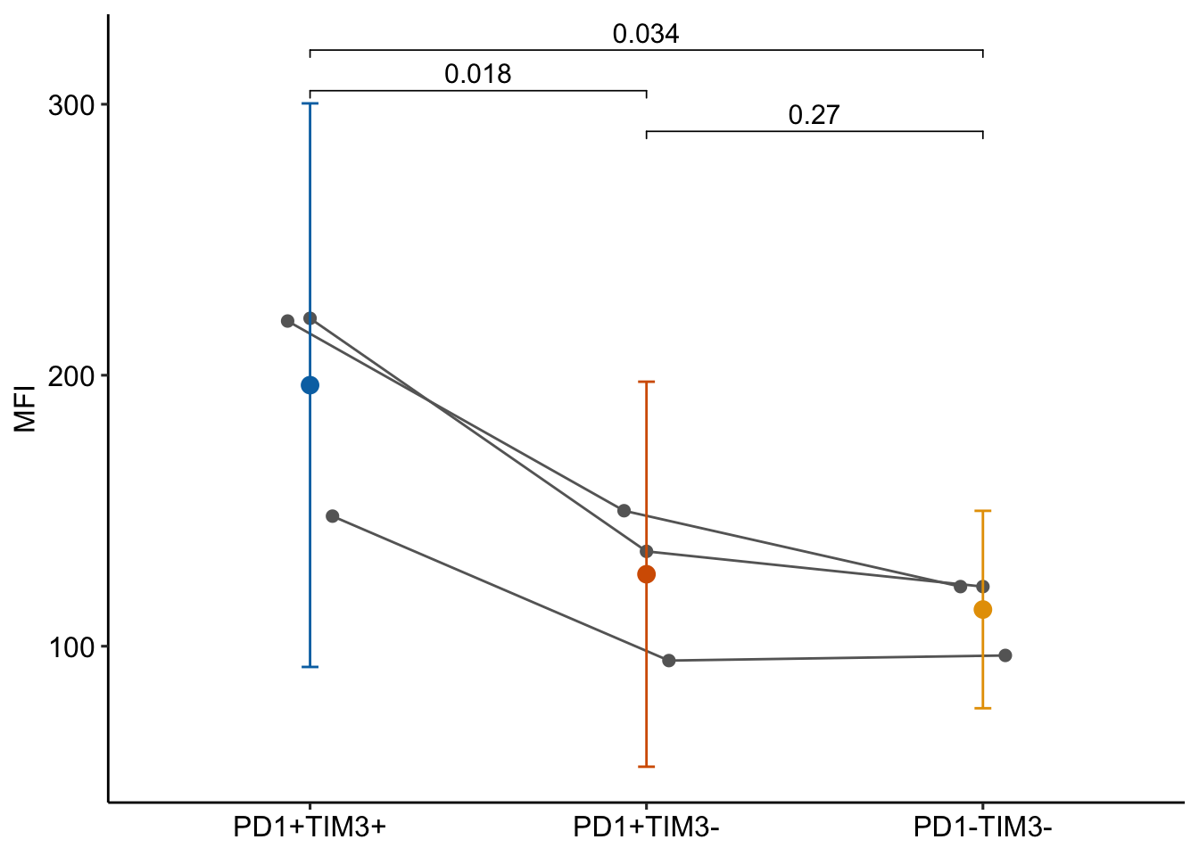
16.15.1.2 Models with subsampling - Experiment 1g
Data wrangling necessary for plot:
# add treatment column to emmeans table
exp1g_m1_emm_dt <- summary(exp1g_m1_emm) |>
  data.table()
exp1g_m1_emm_dt[, treatment := paste(genotype, sex)]
exp1g_m1_emm_dt[, treatment := factor(treatment,
                                      levels = levels(exp1g$treatment))]

# create table of means for each treatment * experiment_id combination
exp1g[, group_mean := predict(exp1g_m1)]
exp1g_m1_emm2 <- exp1g[, .(group_mean = mean(group_mean)),
                       by = .(treatment, experiment_id)]

# add group1 and group2 columns to exp1g_m1_planned
exp1g_m1_planned_dt <- data.table(exp1g_m1_planned)
exp1g_m1_planned_dt[, pretty_p := pvalString(p.value)]
exp1g_m1_planned_dt[, group1 := c("Gpr174- M", "Gpr174- F", "")]
exp1g_m1_planned_dt[, group2 := c("Gpr174+ M", "Gpr174+ F", "")]
# get coefficients of model
b <- exp1g_m1_coef[, "Estimate"]
# get interaction p
p_ixn <- exp1g_m1_planned_dt[contrast == "Interaction", pretty_p]
exp1g_plot_a <- ggplot(data = exp1g,
aes(x = treatment,
y = gc,
color = experiment_id)) +
# modeled experiment by treatment means
geom_point(data = exp1g_m1_emm2,
aes(y = group_mean,
color = experiment_id),
position = position_dodge(width = 0.4),
alpha = 1,
size = 2) +
geom_line(data = exp1g_m1_emm2,
aes(y = group_mean,
group = experiment_id,
color = experiment_id),
position = position_dodge(width = 0.4)) +
# raw data
geom_point(position = position_dodge(width = 0.4),
alpha = 0.3
) +
# modeled treatment means
geom_point(data = exp1g_m1_emm_dt,
aes(x = treatment,
y = emmean),
color = "black",
size = 3) +
# geom_errorbar(data = exp1g_m1_emm_dt,
# aes(y = emmean,
# ymin = lower.CL,
# ymax = upper.CL),
# color = "black",
# width = .05) +
# pvalue brackets
stat_pvalue_manual(exp1g_m1_planned_dt[1:2],
label = "pretty_p",
y.position = c(20,20),
size = 2.5,
tip.length = 0.01) +
# additive line + interaction p bracket
geom_segment(x = 3.85,
y = b[1] + b[2] + b[3],
xend = 4.15,
yend = b[1] + b[2] + b[3],
linetype = "dashed",
color = "gray") +
geom_bracket(
x = 4.2,
y = b[1] + b[2] + b[3],
yend = b[1] + b[2] + b[3] + b[4],
label = paste0("interaction\np = ", p_ixn),
text.size = 3,
text.hjust = 0,
color = "black") +
ylab("GC (%)") +
scale_color_manual(values = pal_okabe_ito_blue) +
theme_pubr() +
coord_cartesian(xlim = c(1, 4.1)) +
theme(
axis.title.x = element_blank(), # no x-axis title
legend.position = "none"
) +
NULL
exp1g_plot_a <- factor_wrap(exp1g_plot_a)
#exp1g_plot_a# get coefficients of model
b <- exp1g_m1_coef[, "Estimate"]
# get interaction p
p_ixn <- exp1g_m1_planned_dt[contrast == "Interaction", pretty_p]
dodge_width = 0.6
exp1g_plot_b <- ggplot(data = exp1g,
aes(x = treatment,
y = gc,
color = experiment_id)) +
# modeled experiment by treatment means
geom_point(data = exp1g_m1_emm2,
aes(y = group_mean,
color = experiment_id),
position = position_dodge(width = dodge_width),
alpha = 1,
size = 2) +
geom_line(data = exp1g_m1_emm2,
aes(y = group_mean,
group = experiment_id,
color = experiment_id),
position = position_dodge(width = dodge_width)) +
# raw data
geom_point(position = position_dodge(width = dodge_width),
color = "gray80"
) +
# modeled treatment means
geom_point(data = exp1g_m1_emm_dt,
aes(x = treatment,
y = emmean),
color = "black",
size = 3) +
# geom_errorbar(data = exp1g_m1_emm_dt,
# aes(y = emmean,
# ymin = lower.CL,
# ymax = upper.CL),
# color = "black",
# width = .05) +
# pvalue brackets
stat_pvalue_manual(exp1g_m1_planned_dt[1:2],
label = "pretty_p",
y.position = c(20,20),
size = 2.5,
tip.length = 0.01) +
# additive line + interaction p bracket
geom_segment(x = 4 - dodge_width/2,
y = b[1] + b[2] + b[3],
xend = 4 + dodge_width/2,
yend = b[1] + b[2] + b[3],
linetype = "dashed",
color = "gray") +
geom_bracket(
x = 4 + dodge_width/1.9,
y = b[1] + b[2] + b[3],
yend = b[1] + b[2] + b[3] + b[4],
label = paste0("interaction\np = ", p_ixn),
text.size = 3,
text.hjust = 0,
color = "black") +
ylab("GC (%)") +
scale_color_manual(values = pal_okabe_ito_blue) +
theme_pubr() +
coord_cartesian(xlim = c(1, 4.2)) +
theme(
axis.title.x = element_blank(), # no x-axis title
legend.position = "none"
) +
NULL
exp1g_plot_b <- factor_wrap(exp1g_plot_b)
# exp1g_plot_b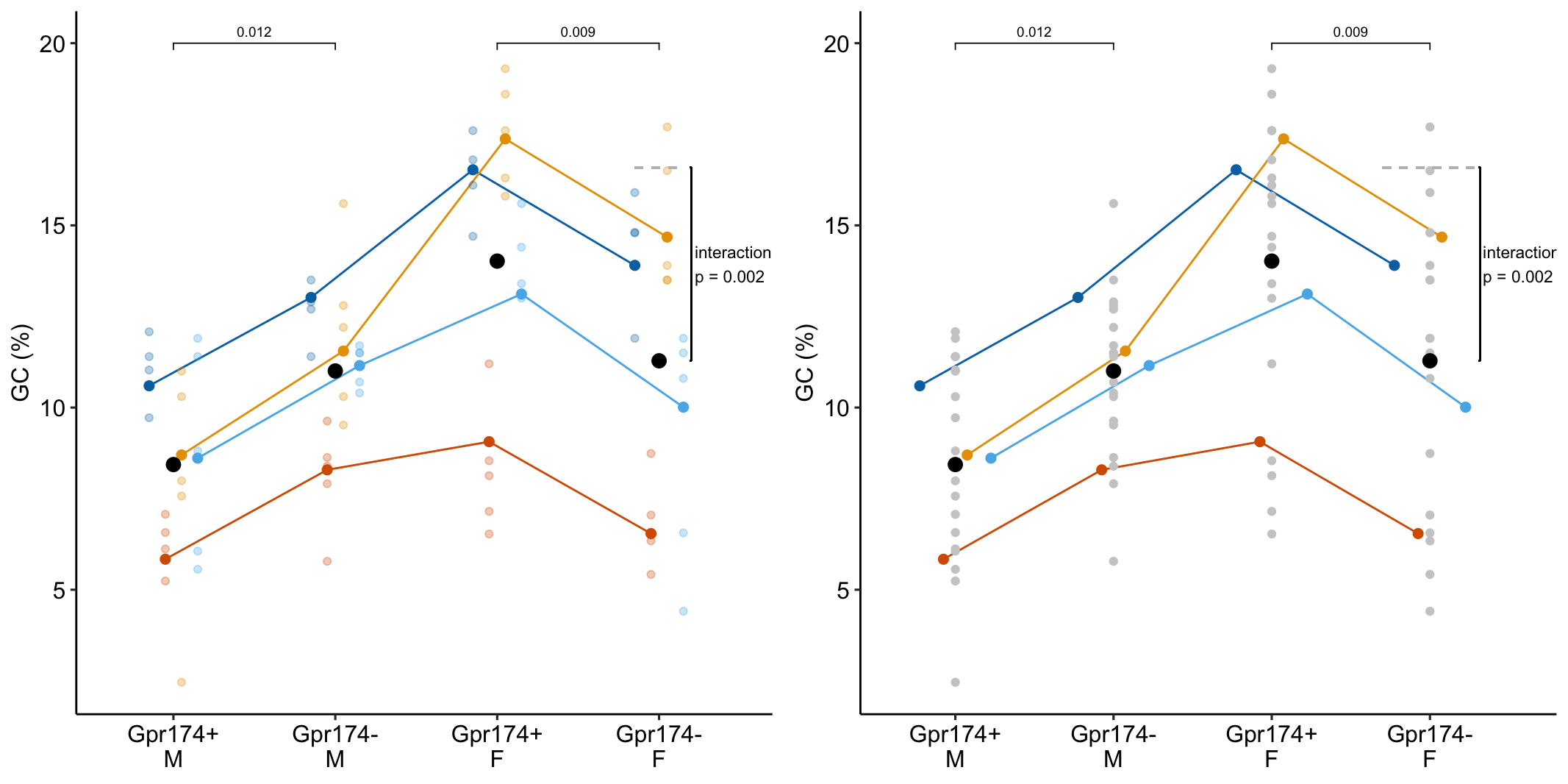
16.15.2 Repeated measures ANOVA (randomized complete block with no subsampling)
# this is the rm-ANOVA
m1 <- aov_4(glucose_uptake ~ treatment * activity +
              (treatment * activity | donor),
            data = fig5c)

# lmm equivalent

m2 <- lmer(glucose_uptake ~ treatment * activity +
         (1 | donor) +
         (1 | donor:treatment) +
         (1 | donor:activity),
       data = fig5c)

# random intercept and slope model that is *not* equivalent
# this isn't solvable because there is no subsampling

m3 <- lmer(glucose_uptake ~ treatment * activity +
              (treatment * activity | donor),
            data = fig5c)
Notes
afexcomputes the repeated measures anova model using bothaov(classical univariate repeated measures ANOVA) and usinglmwith multiple response variables (the multivariate repeated measures ANOVA). As of this writing, the output fromaovis the default.- Given only one measure for each donor within a \(\texttt{treatment} \times \texttt{activity}\) combination, the linear mixed model
m2is equivalent to the univariate repeated measures model m1. - The model formula in
m1looks like that in the linear mixed modelm3but the two models are not equivalent.
16.15.2.1 univariate vs. multivariate repeated measures ANOVA
Use the multivariate model unless you want to replicate the result of someone who used a univariate model. By default, aov_4 computes only the multivariate model (prior to version xxx, the default was to compute both models).
# default mode -- should be multivariate
fig5c_aov <- aov_4(glucose_uptake ~ treatment * activity +
                    (treatment * activity | donor),
                  data = fig5c)

# force aov_4 to compute univariate model
fig5c_rmaov.mul <- aov_4(glucose_uptake ~ treatment * activity +
                    (treatment * activity | donor),
                  data = fig5c,
                  include_aov = TRUE)

# explicitly exclude the univariate model
fig5c_aov1 <- aov_4(glucose_uptake ~ treatment * activity +
                    (treatment * activity | donor),
                  data = fig5c,
                  include_aov = FALSE)
Notes
- The
include_aov = TRUEargument forces output fromaov_4to include the univariate model.
contrasts from multivariate model
# These three should give equivalent results

# fig5c_aov was fit with the default -- multivariate model only
emmeans(fig5c_aov,
        specs = c("treatment", "activity")) |>
  contrast(method = "revpairwise",
           simple = "each",
           combine = TRUE,
           adjust = "none")
activity treatment contrast estimate SE df t.ratio p.value
Basal . siNR4A3 - Scr 0.0813 0.1010 5 0.804 0.4581
EPS . siNR4A3 - Scr -0.1858 0.0359 5 -5.180 0.0035
. Scr EPS - Basal 0.1510 0.0395 5 3.821 0.0124
. siNR4A3 EPS - Basal -0.1161 0.0626 5 -1.855 0.1228# fig5c_aov included the univariate model but the default is still the multivariate model
emmeans(fig5c_rmaov.mul,
specs = c("treatment", "activity")) |>
contrast(method = "revpairwise",
simple = "each",
combine = TRUE,
adjust = "none") activity treatment contrast estimate SE df t.ratio p.value
Basal . siNR4A3 - Scr 0.0813 0.1010 5 0.804 0.4581
EPS . siNR4A3 - Scr -0.1858 0.0359 5 -5.180 0.0035
. Scr EPS - Basal 0.1510 0.0395 5 3.821 0.0124
. siNR4A3 EPS - Basal -0.1161 0.0626 5 -1.855 0.1228# passing `model = "multivariate"` makes the model choice transparent
emmeans(fig5c_rmaov.mul,
specs = c("treatment", "activity"),
model = "multivariate") |>
contrast(method = "revpairwise",
simple = "each",
combine = TRUE,
adjust = "none") activity treatment contrast estimate SE df t.ratio p.value
Basal . siNR4A3 - Scr 0.0813 0.1010 5 0.804 0.4581
EPS . siNR4A3 - Scr -0.1858 0.0359 5 -5.180 0.0035
. Scr EPS - Basal 0.1510 0.0395 5 3.821 0.0124
. siNR4A3 EPS - Basal -0.1161 0.0626 5 -1.855 0.1228Notes
- If our rmANOVA model is fit with the default specification (
fig5c_rmaov.mul), we can get the multivariate output using themodel = "multivariate"argument withinemmeans(not thecontrastfunction!). Or, if our fit excluded the univariate model (fig5c_aov1), then we don’t need themodelargument.
contrasts from univariate model
# get the univariate model results using $aov
emmeans(fig5c_rmaov.mul$aov, specs = c("treatment", "activity")) |>
  contrast(method = "revpairwise",
           simple = "each",
           combine = TRUE,
           adjust = "none")
activity treatment contrast estimate SE df t.ratio p.value
Basal . siNR4A3 - Scr 0.0813 0.0759 8.60 1.071 0.3132
EPS . siNR4A3 - Scr -0.1858 0.0759 8.60 -2.448 0.0380
. Scr EPS - Basal 0.1510 0.0524 9.39 2.884 0.0173
. siNR4A3 EPS - Basal -0.1161 0.0524 9.39 -2.218 0.0525Notes
- Passing
fig5c_rmaov.multoemmeanswill return the contrasts from the multivariate. change this to the univariate model by passingfig5c_rmaov.mul$aov.
16.15.2.2 The ANOVA table
nice(fig5c_rmaov.mul, correction = "GG")Anova Table (Type 3 tests)
Response: glucose_uptake
Effect df MSE F ges p.value
1 treatment 1, 5 0.02 0.68 .006 .448
2 activity 1, 5 0.01 0.30 <.001 .609
3 treatment:activity 1, 5 0.01 10.37 * .037 .023
---
Signif. codes: 0 '***' 0.001 '**' 0.01 '*' 0.05 '+' 0.1 ' ' 1nice(fig5c_rmaov.mul, correction = "none")Anova Table (Type 3 tests)
Response: glucose_uptake
Effect df MSE F ges p.value
1 treatment 1, 5 0.02 0.68 .006 .448
2 activity 1, 5 0.01 0.30 <.001 .609
3 treatment:activity 1, 5 0.01 10.37 * .037 .023
---
Signif. codes: 0 '***' 0.001 '**' 0.01 '*' 0.05 '+' 0.1 ' ' 1Notes
- The Greenhouse-Geiger (“GG”) correction is the default. While the
correction = "GG"argument is not needed, it makes the script more transparent. - For these data the Greenhouse-Geiger correction doesn’t make a difference in the table.
16.15.2.3 Split plot simulation
Performance:
| sim_id | sig_block | sig_ss | sig_main | sig_sub | contrast | r | lm.crd | lm.fe | lmm.ri | lmm.ris | lmm.rii | lmm5 | lmm.sp1 |
|---|---|---|---|---|---|---|---|---|---|---|---|---|---|
| sim 1 - block:main plot | |||||||||||||
| 1 | 0.8 | 0.5 | 0.6 | 0.0 | main | 0.494 | 0.083 | ||||||
| 1 | 0.8 | 0.5 | 0.6 | 0.0 | sub | 0.783 | 0.011 | ||||||
| sim 2 - block:sub plot | |||||||||||||
| 2 | 0.8 | 0.5 | 0.0 | 0.6 | main | 0.782 | 0.042 | ||||||
| 2 | 0.8 | 0.5 | 0.0 | 0.6 | sub | 0.497 | 0.050 | ||||||
| sim 3 - block:main + block:sub | |||||||||||||
| 3 | 0.8 | 0.5 | 0.6 | 0.4 | main | 0.549 | 0.068 | ||||||
| 3 | 0.8 | 0.5 | 0.6 | 0.4 | sub | 0.689 | 0.024 | ||||||
| sim 4 - block only | |||||||||||||
| 4 | 0.8 | 0.5 | 0.0 | 0.0 | main | 0.707 | 0.056 | ||||||
| 4 | 0.8 | 0.5 | 0.0 | 0.0 | sub | 0.704 | 0.052 | ||||||